Space Weather JHelioviewer is an outcome of the ESA Contract No. 4000107325/12/NL/AK - High Performance Distributed Solar Imaging and Processing System - run at the Solar Influences Data Analysis Center (SIDC) of the Royal Observatory of Belgium (ROB). This project is part of the ESA/NASA Helioviewer Project (https://helioviewer.org).
The JHelioviewer solar data visualisation tool has been overhauled with a strong focus for space weather usage. The viewer is able to display solar image data, and one-dimensional and two-dimensional solar timeline data.
The solar images can be projected on a sphere. They can be rotated, translated, and zoomed in and out the sphere. Other projections are available, such as solar latitudinal or (log)polar. Field lines of the solar magnetic field calculated by a PFSS model can be displayed.
The timeline viewer shows one-dimensional and two-dimensional data. The time interval displayed can be translated and zoomed freely.
Several types of space weather related events can be displayed. Both the Heliophysics Events Knowledgebase and the COMESEP project provide the events. The events can be visualised on both the images and the timelines.
Since JHelioviewer is still rapidly evolving, this document may not reflect entirely all the capabilities of the software. Information and support requests can be sent to swhv@sidc.be.
The JHelioviewer software does advanced data processing and visualisation; therefore it works best on a reasonably recent computer with decent CPU and OpenGL graphics power, and memory. It contains native compiled libraries to speed up critical operations. The supported computer architecture are Intel/AMD 64-bit and, on macOS, Apple Silicon (ARM64). The minimal OpenGL version required is 3.3.
JHelioviewer is an open source project and its source code can be accessed at https://github.com/Helioviewer-Project/JHelioviewer-SWHV.
Compiled releases are available for Windows, macOS and Linux from https://swhv.oma.be/download. A brief changelog is at https://github.com/Helioviewer-Project/JHelioviewer-SWHV/blob/master/changelog.md.
dpkg -i JHelioviewer_*_amd64.deb or rpm --install JHelioviewer_*_amd64.rpm with supervisor privileges.jhelioviewer in a terminal window. For correct UI scaling on HiDPI displays use jhelioviewer -J-Dsun.java2d.uiScale=2 and replace 2 with the scaling factor of your display.java --add-exports java.desktop/sun.awt=ALL-UNNAMED --add-exports java.desktop/sun.swing=ALL-UNNAMED -cp JHelioviewer.jar:natives-linux.jar:natives-macos.jar:natives-windows.jar org.helioviewer.jhv.JHelioviewer in a terminal window.This procedure works for Windows, macOS and Linux.
The program accepts command line arguments. This is implemented using JSON documents specifying requests to the default server in a simple manner as in the example below. Natural language specification of time is supported (as is the case for the state file) and, besides the “dataset” field, all fields are optional with sensible defaults.
{
    "observatory": "SDO",
    "startTime": "yesterday",
    "endTime": "today",
    "cadence": 1800,
    "dataset": "AIA 304"
}
When the program opens for the first time, a directory structure (JHelioviewer-SWHV) is created in the home directory. It contains configuration files, exported movies, plugins and other data.
The Troubleshooting and Frequent Asked Questions sections may contain contain useful hints about installing and running JHelioviewer.
The following YouTube video demonstrates some basic functionalities of the interface.
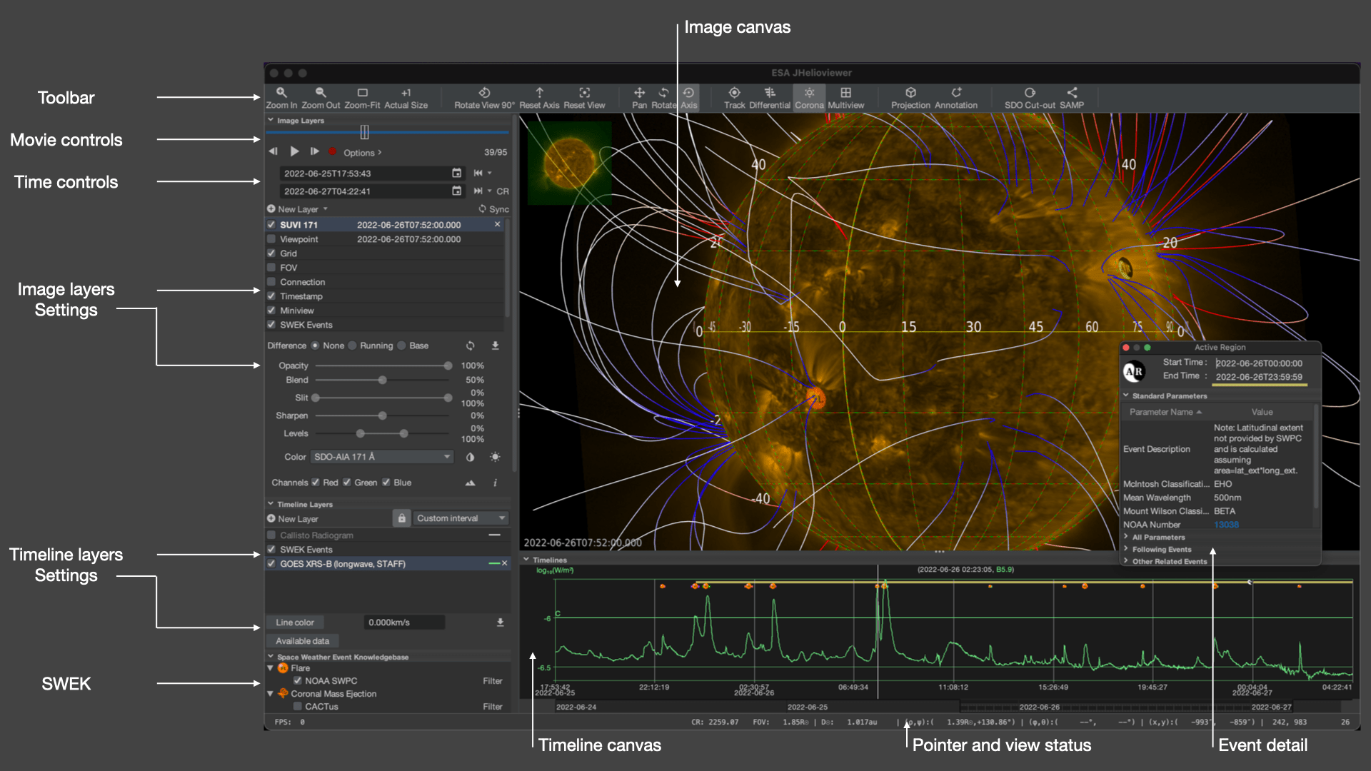
The main user interface consists of the toolbar, the image canvas, the timeline canvas, the control panels, the view status and the mouse position indicators.
The toolbar is divided into three parts: the camera controlling part, the image controlling part and the four distinct miscellaneous parts. The camera controlling part allows to zoom in and out the image, fit the image in the available canvas, show the image at full scale (one image pixel corresponding to one pixel on screen), and reset the camera back into its original orientation.
The image on the image canvas can be rotated, rotated around the axis, translated and annotated. Each of those interaction modes can be enabled in the image controlling part of the toolbar.
The miscellaneous part of the toolbar contains buttons to switch on and off the solar rotation tracking and the visibility of off-disk corona. The corona button hides the off-disk corona from the images, while the solar rotation tracking button fixes the camera orientation and co-rotates with the Sun while the movie is played.
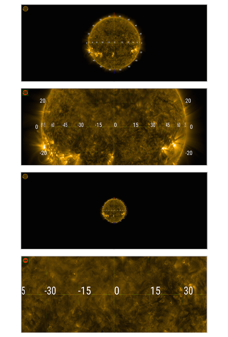
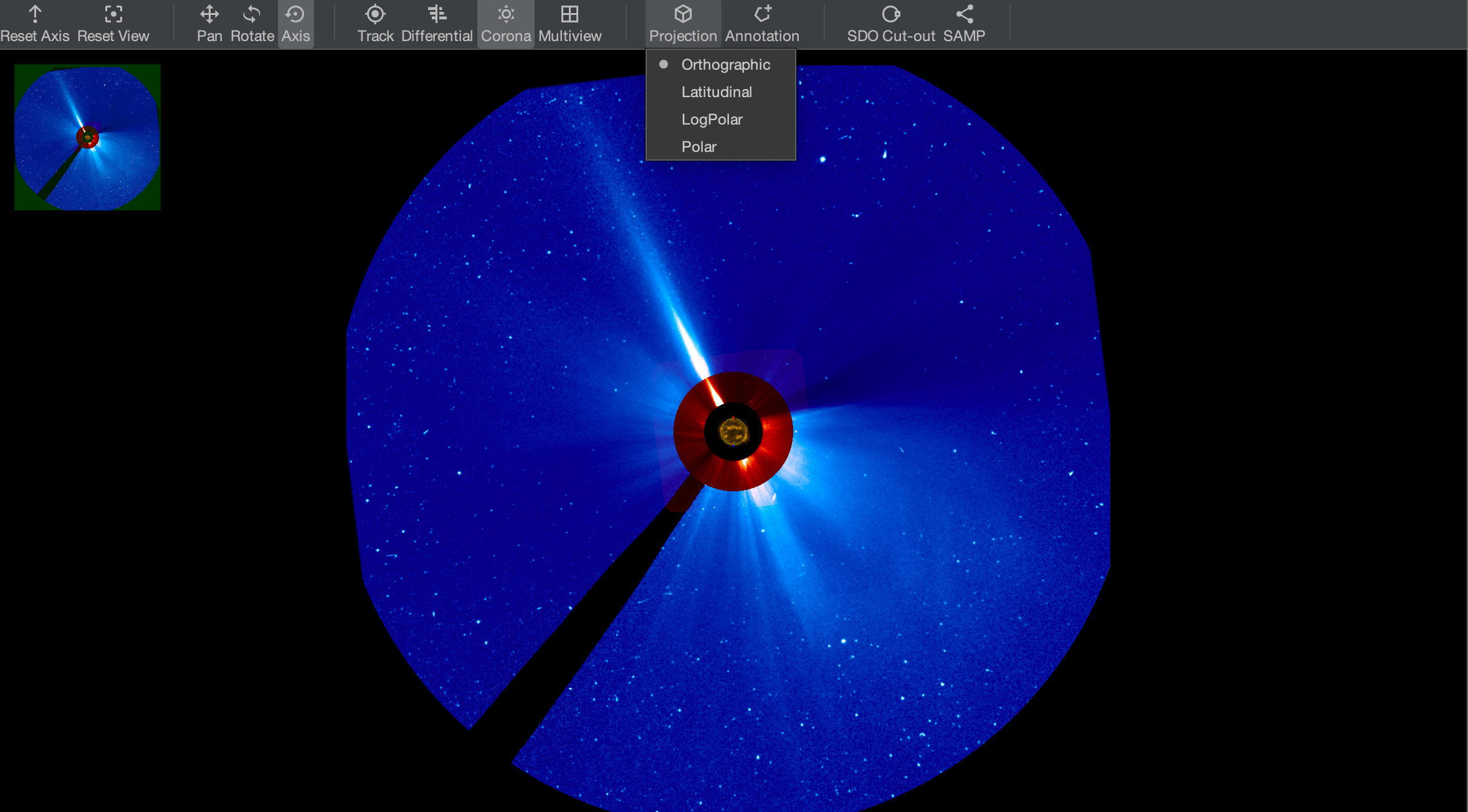
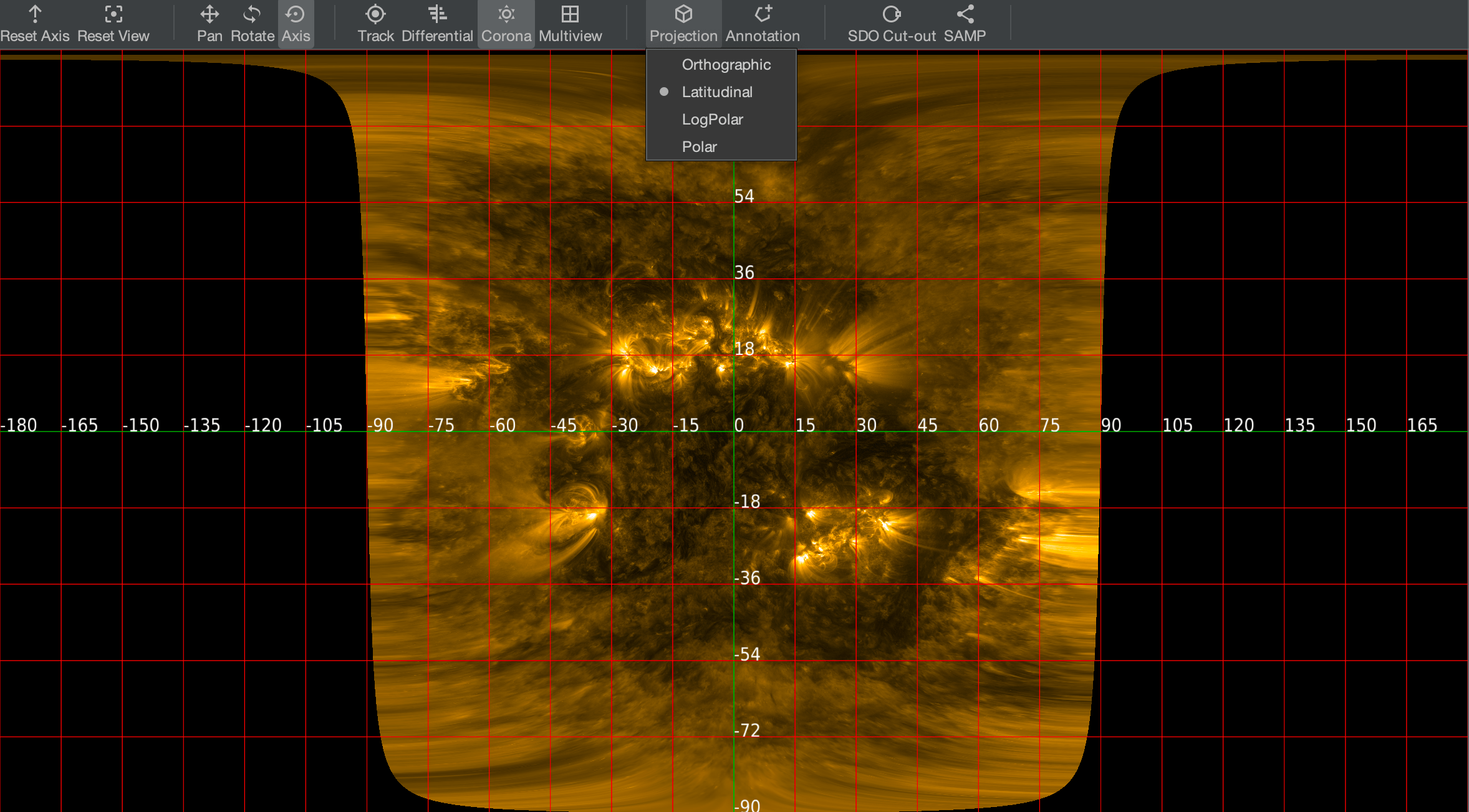
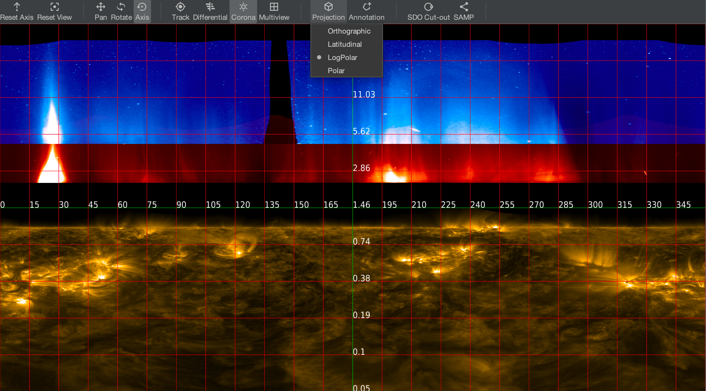
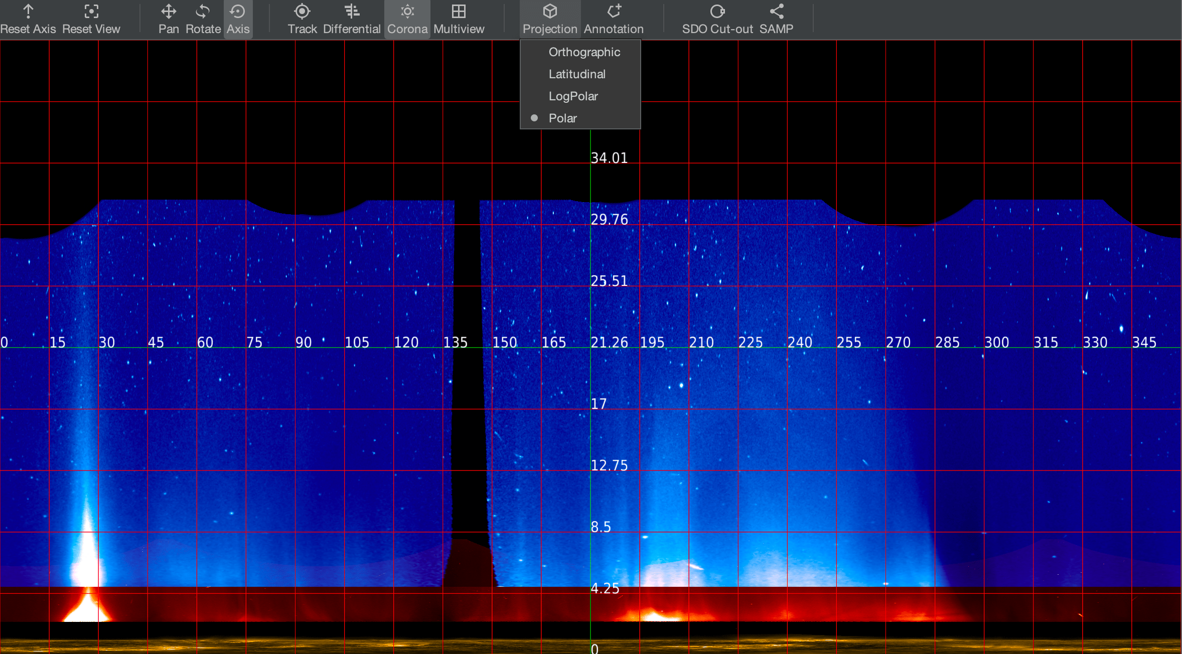
The image canvas displays in four projections: the default orthographic, latitudinal, logpolar and polar projection. Switching from one projection to the other is instantaneous.
There is also a direct link to the SDO AIA get data page (https://www.lmsal.com/get_aia_data/).
The data of the image layer can be broadcasted using the Simple Application Message Protocol(SAMP).
See the image canvas manipulation section and the toolbar figure for all the functionalities.
The image canvas displays the visible image layers. The images of the Sun are projected on a sphere. As long as no manipulations to the scene are done, and the viewpoint is not altered, the image is an undistorted representation of the two-dimensional data recorded by the instrument.
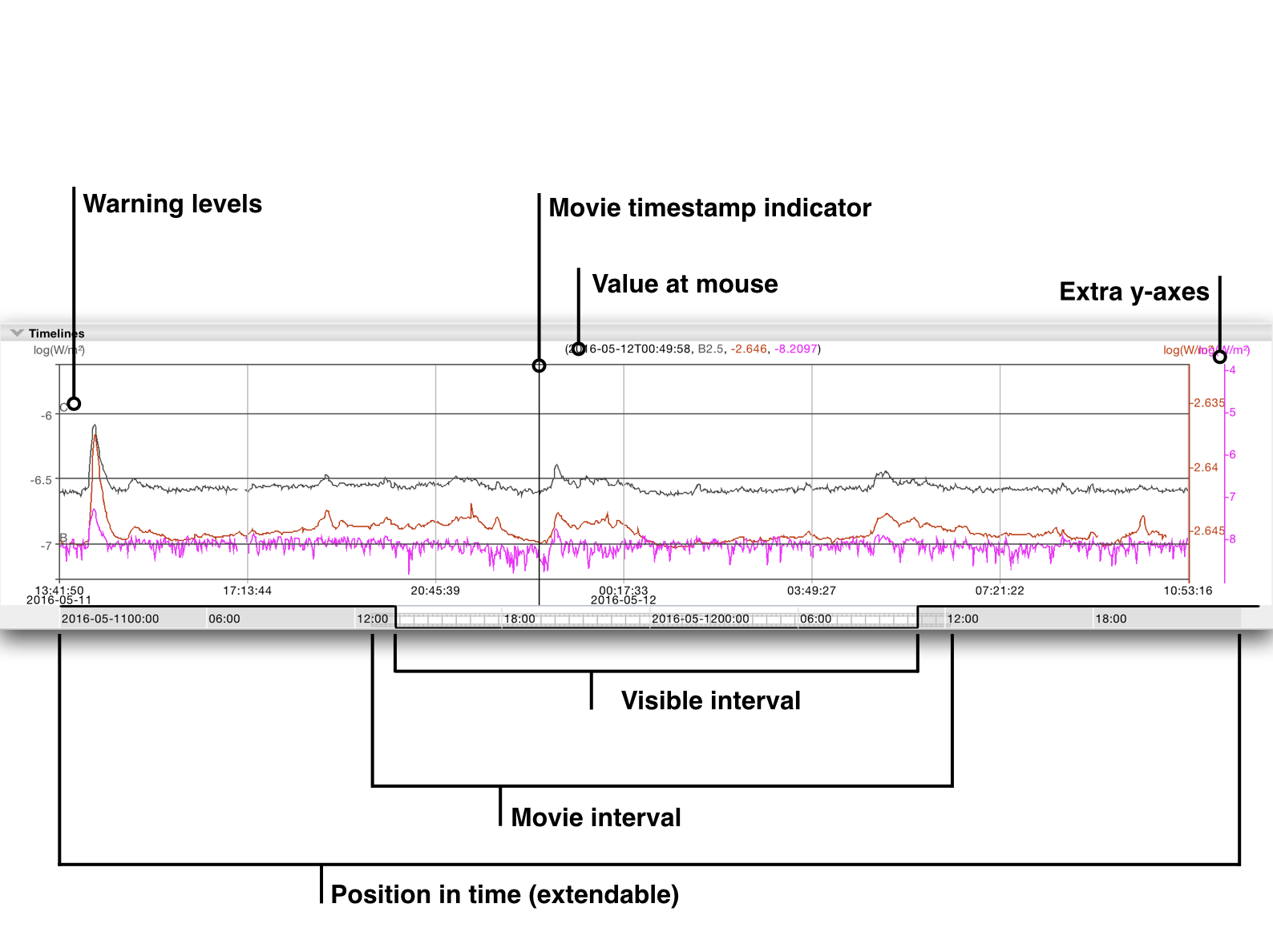
The timeline canvas shows timelines and radio spectrograms (see the timeline figure). The timeline canvas can have multiple y-axes. It can display multiple timelines and space weather events. The time handling section visualises the position in time, the movie interval and the visible interval.
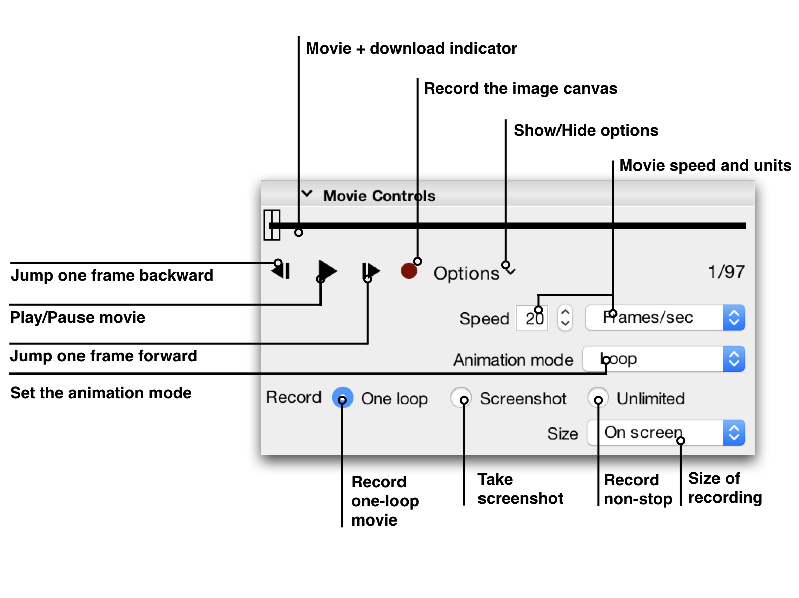
The movie controls allow playing and pausing the current movie. The movie can be advanced by one frame at a time in forward or backward direction. The image canvas can be recorded (see the section on recording). The movie controls have additional options where the frame rate, animation mode, and the recording mode and size can be set.
The image layers panel provides an overview of the image layers and the options of the selected layer. Information about the layers is given in the table listing. Some layers can be deleted; all layers can be made visible or invisible. The visible layers will be displayed on the image canvas. Every layer has specific options that become available if the corresponding entry in the table is selected. New image layers can be added. The image layer displayed with a bold name is the master image layer. The program time, the movie panel frame indication, and the frame rate displayed by the status indicator are based on the master layer. The full resolution zoom level is also based on the resolution of the master layer. The program attempts to match the frame timestamps of the other image layers to the master layer. Clicking on the name of another image layer leads to the change of the master layer.
The timeline layers panel is similar to the image layers panel. It has two parts: the listing of all the timeline layers and the options attached to the selected timeline layer. Some layers can be deleted; all layers can be made visible or invisible. All visible layers will be displayed on the timeline canvas. Some layers have specific options that become available when the corresponding entry in the table is selected. New timeline layers can be added.
The Space Weather Event Knowledgebase or SWEK offers a list of space weather related event types. Several event types can be enabled. Events for the current period will be downloaded and displayed by the image canvas and the timeline canvas if the corresponding event layers are made visible.
The view status shows the size of the field of view in solar radii, the distance from the Sun, the Carrington rotation number and the current frame rate of image decoding.
The position indicator shows the mouse position in solar coordinates (latitude, longitude) if the mouse pointer hovers over the solar surface, and the plane-of-sky radial distance from the Sun centre.
The image canvas can be manipulated in several ways. It can be zoomed, rotated and translated, the solar rotation can be tracked, the off-disk corona can be made visible or invisible, and the projection can be changed. All those manipulations can be performed from the toolbar as shown in the toolbar figure.
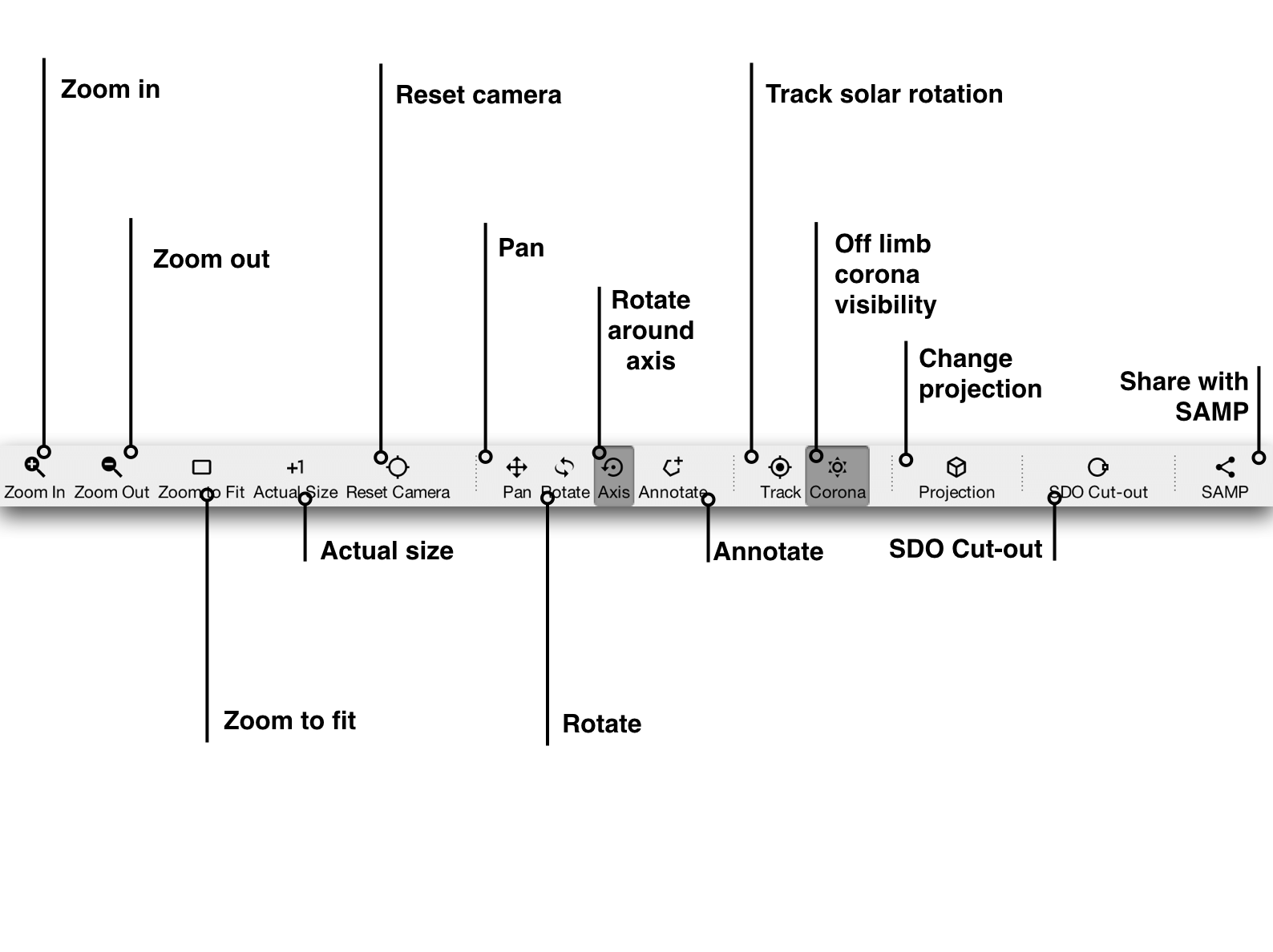
The image can be zoomed by pressing the zoom in and zoom out buttons in the toolbar and also with the mouse by scrolling up and down, or by using the shortcut keys:
The zooming will always take the centre of the image canvas as the focus point. The toolbar figure shows the different zoom options.
The standard mouse operation mode is rotation. By clicking and holding the mouse button, the Sun can be grabbed and rotated freely. By selecting the pan option in the toolbar, clicking and dragging the mouse results in a translation of the image in the image canvas. The figure below shows the result.
It is possible to annotate the image canvas with various shapes. The annotation figure shows an annotated image canvas and the modes when clicking the annotation button. Click the annotate button and select the desired annotation shape. Then press the shift key and drag the mouse pointer with the left button pressed to draw. When finished, release the mouse button, then the shift key. If more than one annotation is added, the red one indicates the active annotation.
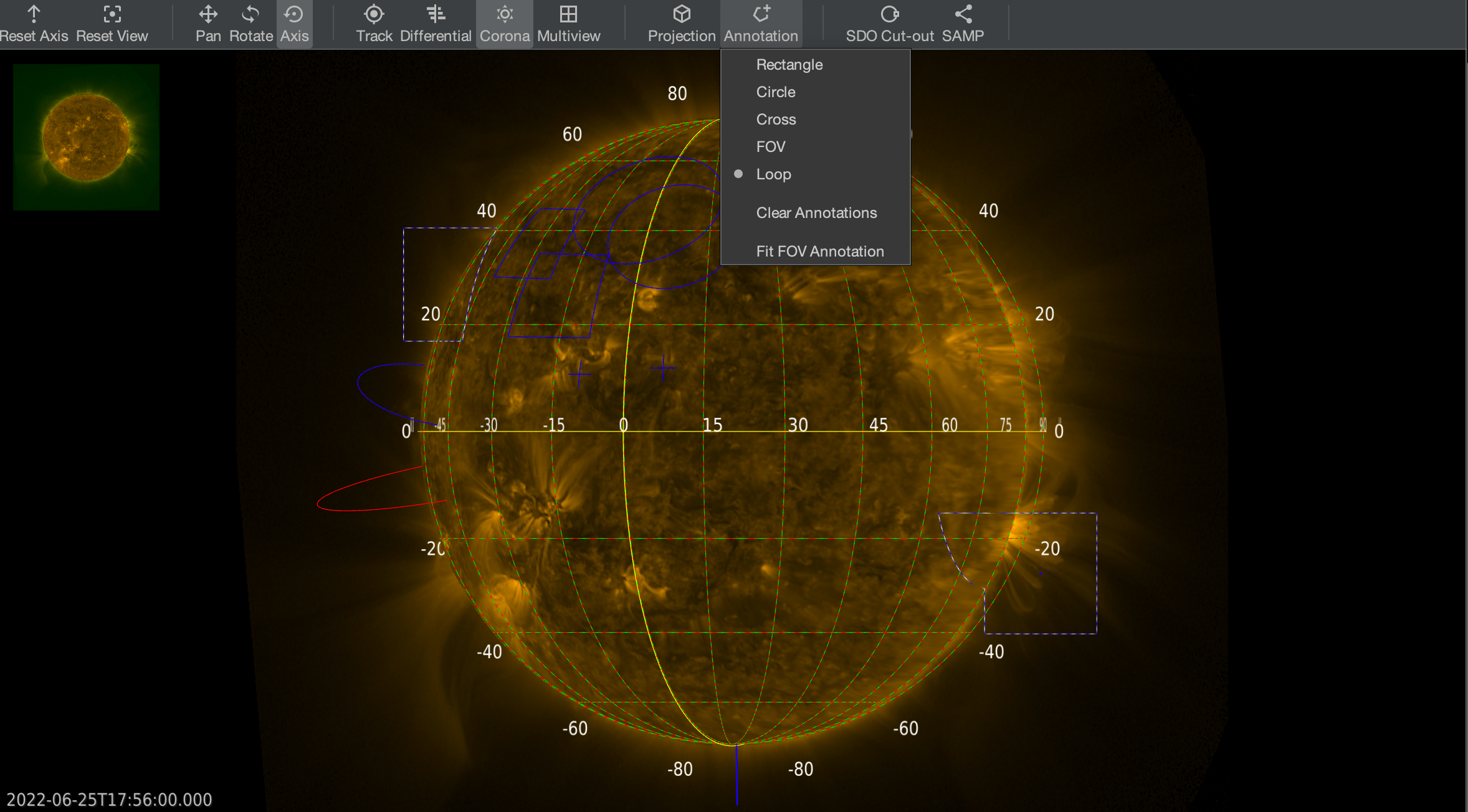
Consider the situation shown by the annotation figure. By pressing shift+n(ext) or shift+p(previous), another annotation will become red. Pressing shift combined with the forward or the backward delete key will delete the red loop. The annotations can deleted all at once via the menu item “View>Clear annotations” or from the toolbar annotation mode button.
The solar rotation can be tracked by freezing the viewpoint time at the moment when the tracking mode is enabled in the toolbar. The image canvas will co-rotate with the Sun when playing the movie, while keeping the original features fixed on screen, allowing to observe their evolution in time.
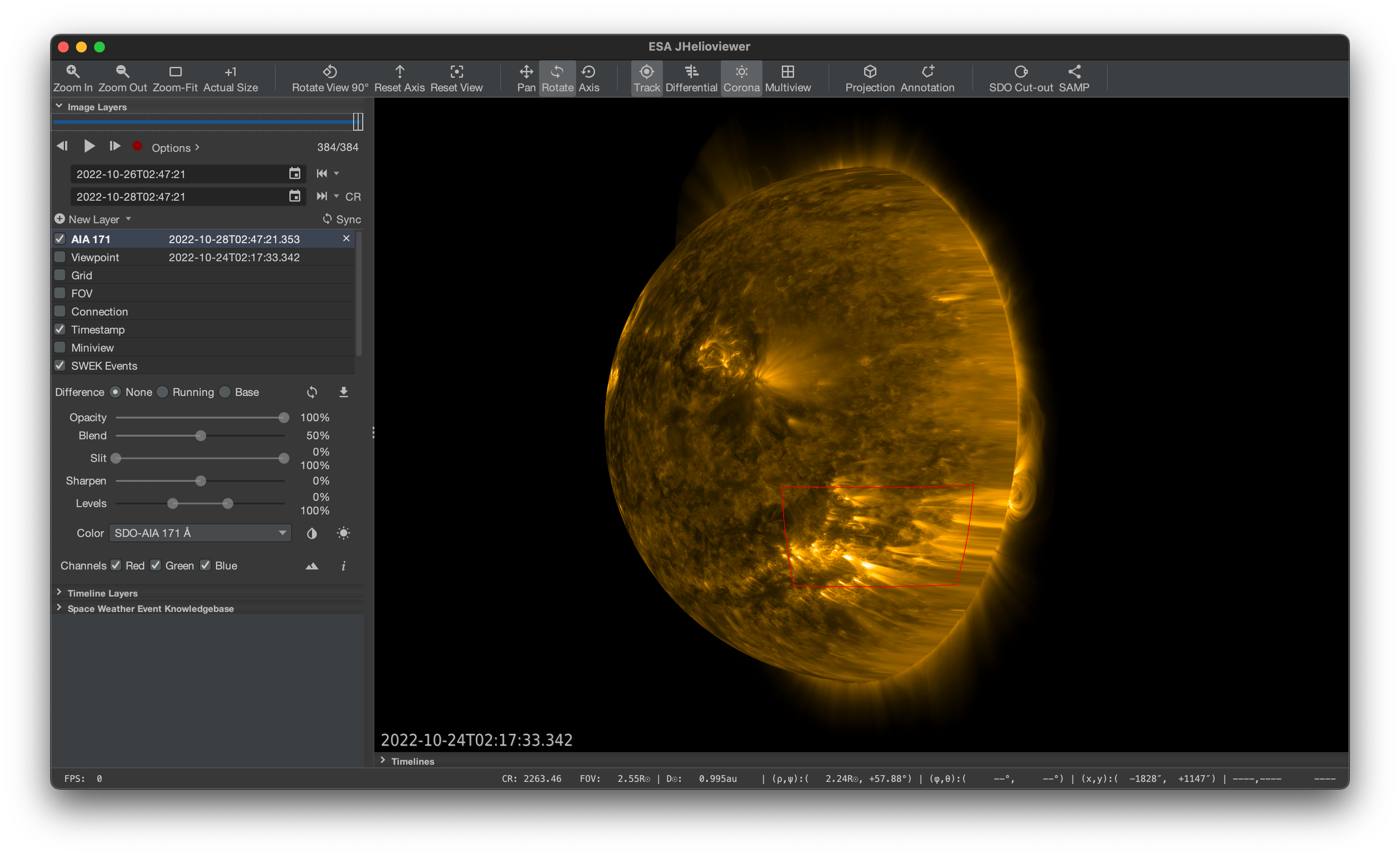
The images can be distorted according to differential solar rotation of magnetic features by selecting the differential option in the toolbar and manipulating the viewpoint time, see viewpoint section.
The off-disk solar corona can hidden by clicking the corona button in the toolbar. The figure below shows the result after turning on this mode.
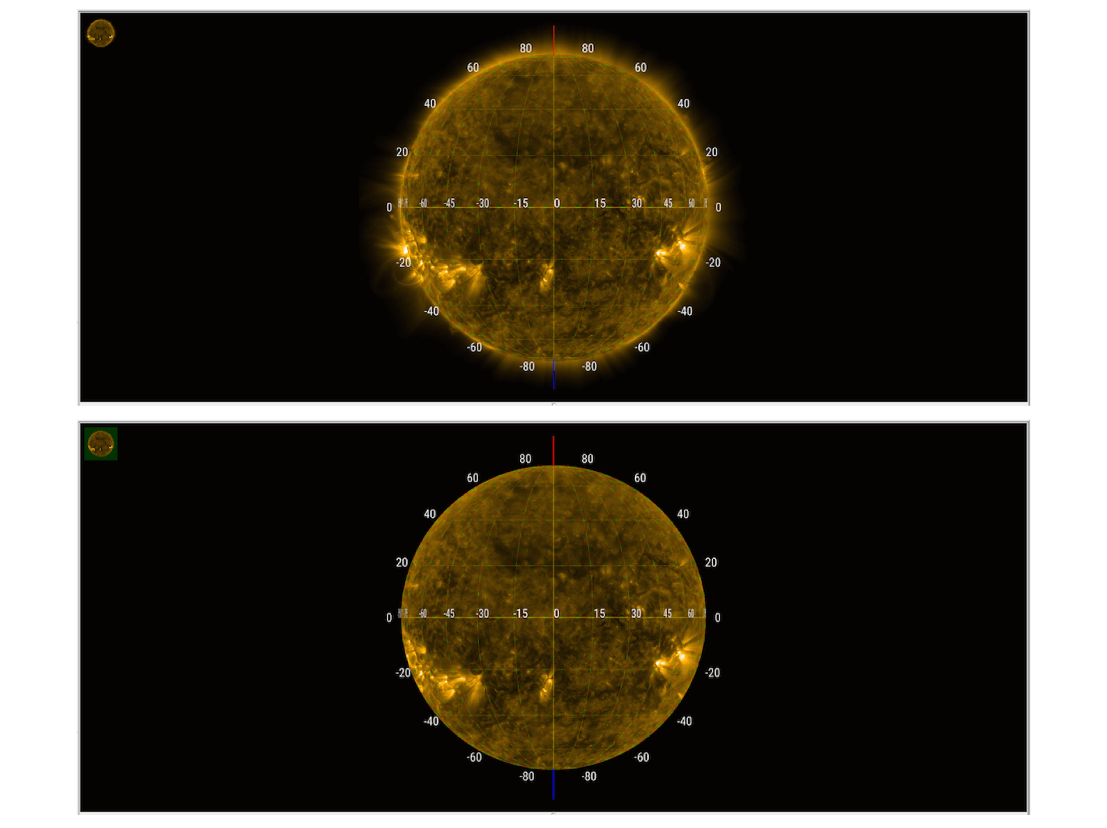
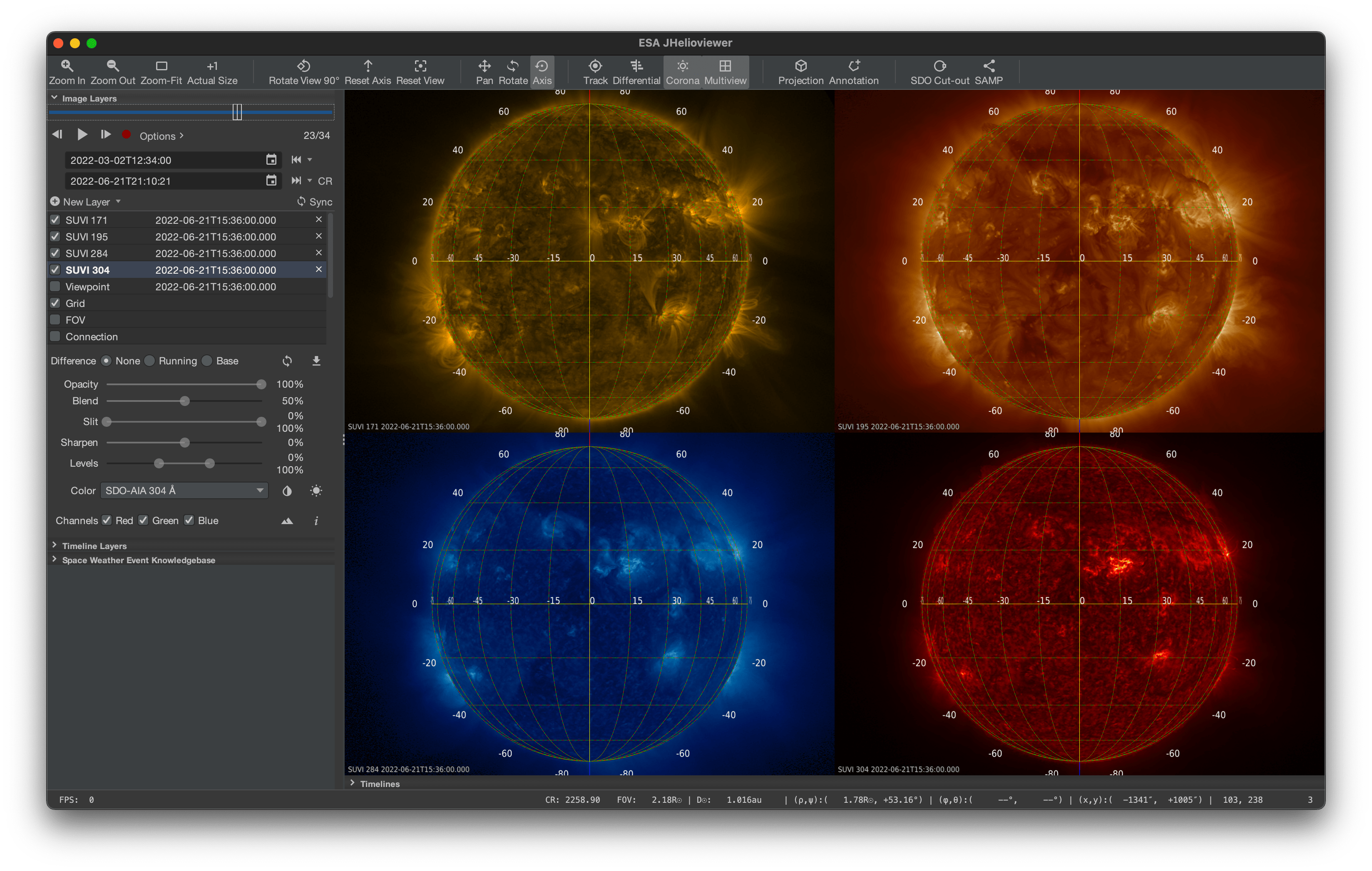
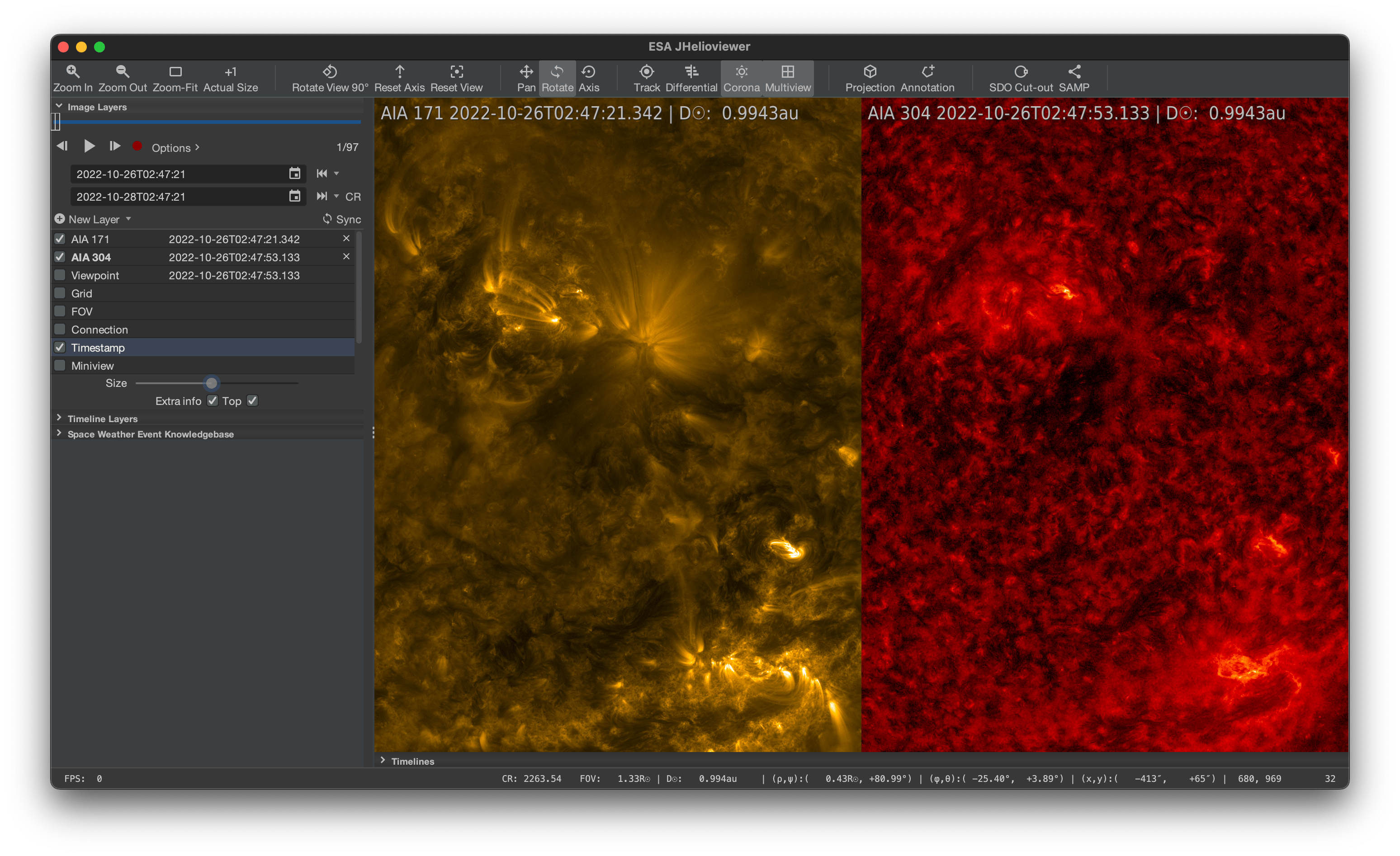
The multiview figure shows what happens if the “Multiview” option in the toolbar is selected. The layers are displayed side-by-side instead of on top of each other. In this mode, up to four layers can be placed together in the image canvas.
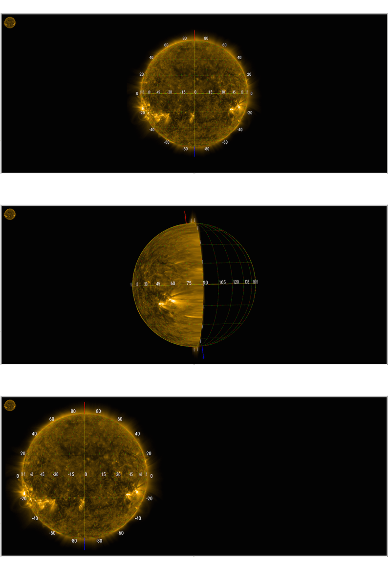
Jhelioviewer is able to show images in four projections: orthographic (default), latitudinal (only for images on the solar disk), logpolar and polar. To change the projection click the projection button in the toolbar and select the projection.
The SDO Cut-out option will open the SDO AIA Get Data page (https://www.lmsal.com/get_aia_data/) at LMSAL with some of the parameters already filled-in based on the current AIA image layer stack.
The movie controls panel contains the tools to play the movie (see the movie panel figure). The movie can be played after at least one image layer with several frames was loaded. The movie is started by pressing the play button or by the ctrl/cmd + p shortcut. The play button becomes a pause button if the movie is playing. The slider visualises in light gray which image frames are partially downloaded and in black which image frames are fully downloaded. The movie can be advanced by one frame at a time in the forward or backward direction by pressing the buttons or by using ctrl/cmd + right arrow and ctrl/cmd + left arrow, respectively. Clicking on the slider or on the timeline canvas allows jumping to arbitrary frames of the movie.
The movie controls panel contains a section with options. The movie options are shown in the movie panel figure. The speed of the movie can be changed, as well as the animation mode from the default loop mode to stop or swing mode. The loop mode will replay the movie from the beginning if the movie reaches the end of the movie, the stop mode will just stop at the end, and the swing mode will play the movie backward and forward again.
The timelines canvas shows the visible timelines. Once a timeline is loaded, it is displayed. The canvas can be translated freely in time by dragging it further to the past or to the future, shift+scroll will do the same. Scrolling on the plotted lines will zoom in time. Holding ctrl while scrolling, or scrolling with the mouse positioned on top of a y-axis will zoom the corresponding values. Clicking and holding the mouse above one the y-axes will translate the y-axis on which the mouse was located. Holding alt while scrolling will zoom both in time and value. Double-clicking the timeline canvas will fit independently the datasets in the plot area. Double-clicking a y-axis will reset its scaling to default.
To zoom in time to some predefined time intervals, like the maximum interval already downloaded, one year, six months, three months, one Carrington rotation, seven days and twelve hours, select one of those options in the dropdown menu located on timeline layers panel. The maximum interval is the interval currently visible in the timeline canvas. Selecting one of the possible periods will increase the interval to the interval of choice while keeping the old intervals upper limit.
Quick jumps to another time are possible by clicking in the interval indicator. The click position will be the centre of the new visible interval.
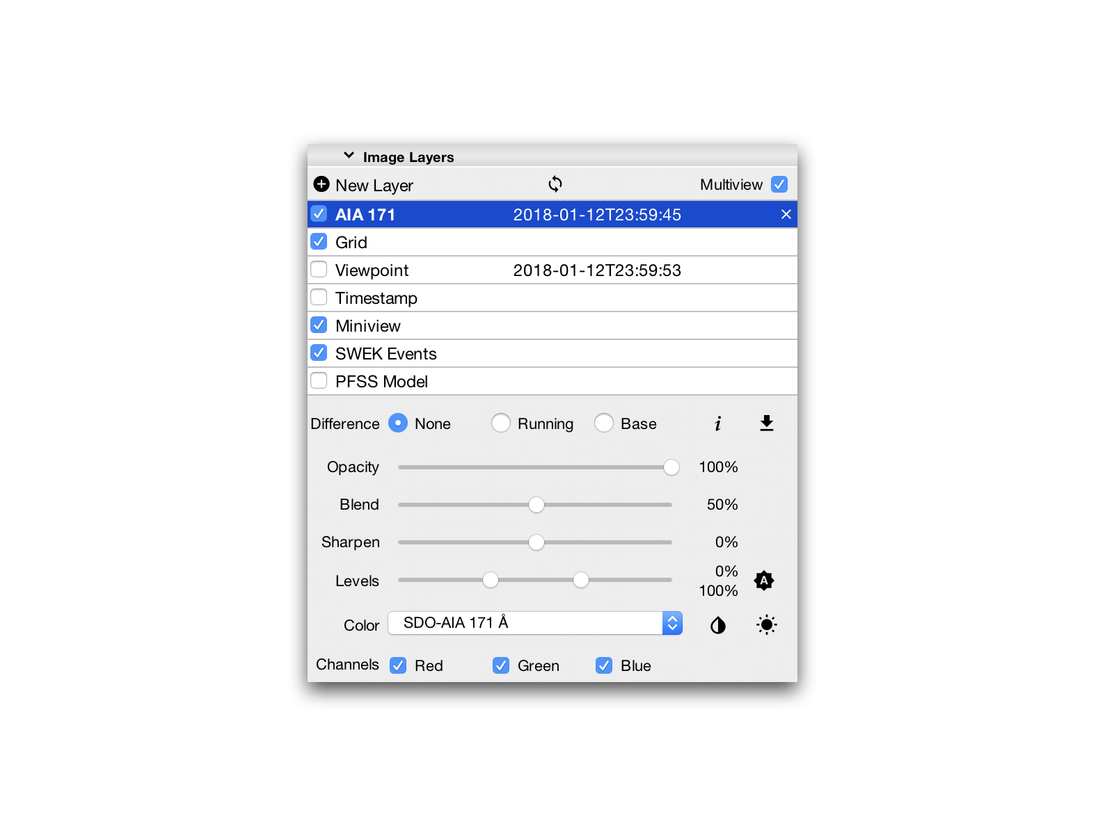
Everything drawn on the image canvas is an image layer. Those layers can be images of the Sun produced by different instruments, a solar grid, a timestamp, a visualisation of a solar magnetic field model (PFSS), the viewpoint, the miniview, and the space weather events (SWEK). The image layers can be deleted by pressing the cross icon, the other layers are fixed and can only be made visible or invisible by pressing the adjacent checkbox. The layers are drawn on the image canvas in the order from the top of the list to the bottom. Dragging and dropping the image layers can change the order.
Each layer has specific options that become available when selecting its entry in the table listing.
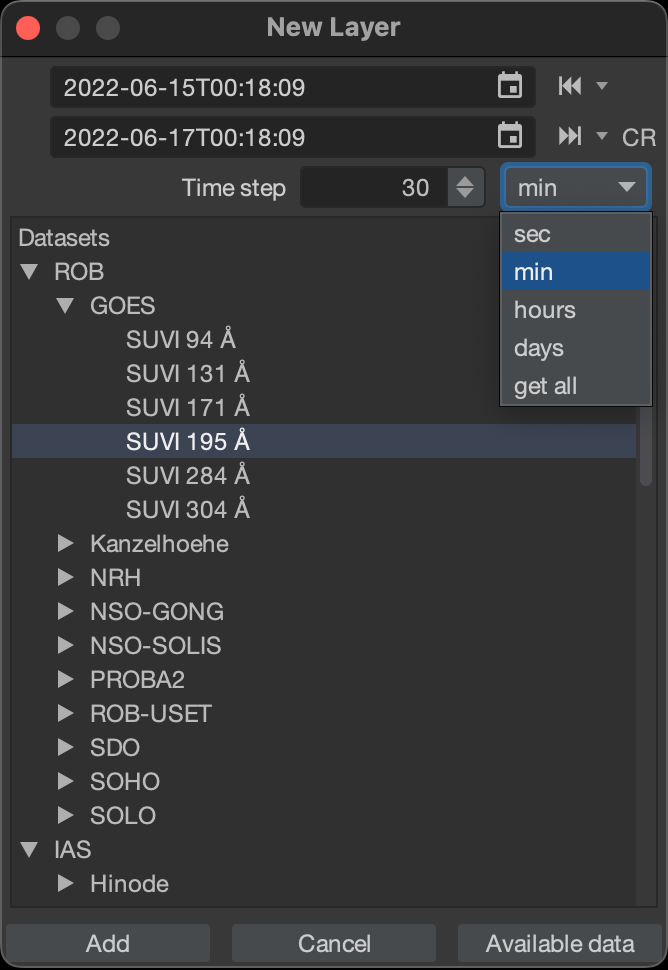
A new image layer can be rapidly added by selecting a time range and clicking “New Layer” in the image layers panel. Select the server from where to download the data, then the dataset from the list.
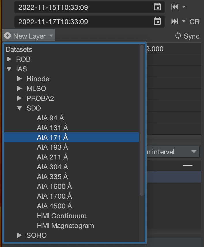
The program calculates a time step for an approximately 98 frames sequence. For control over the cadence, use “File>New Image Layer…” (ctrl/cmd + n) which will open a dialog box where the time step can be changed.
The layer is now added to the list of image layers. The layer becomes the master layer and will drive the timing for playing the movies. A layer can also be added by opening an image or series of images via the menu item “File>Open Image Layer…”. A file selection dialog will open. Select the wanted image or a list of images (using shift for a contiguous list or ctrl/cmd for disjoint list) to be added to the image layers. A list of images can also be added by dragging and dropping from other programs.
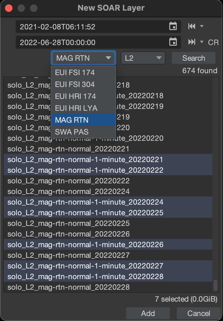
Solar Orbiter science data can also be loaded from the Solar Orbiter Archive at ESAC using the menu item “File>New SOAR Layer…”. Select a time range and search for a dataset and processing level. Select the items to load from the returned list and click the “Add” button. Images will load in the image canvas and time series in the timeline canvas. There is limit of 2GiB data to be loaded at one time.
A layer can be removed by clicking the cross. The loading of a layer can be cancelled by clicking the cross while the layer is still loading.
To change the options of a layer, it has to be selected in the table listing and its options panel will become available underneath the listing. New layers are added with increased levels of transparency to avoid fully concealing the layers beneath and the opacity of each layer can be controlled from its options panel.
Image layers can be replaced by double-clicking in the listing and modifying any of the selection parameters that were initially used. The time span of all image layers loaded can be matched by clicking the “Synchronize layers time span” button.
The availability of image datasets can be checked for the ROB server by clicking on the “Available data” button at the bottom left of the dialog box. A web browser window will open with a page showing an approximation of the available data on the ROB server. The darker the green, the more images are available.
An image layer has several options shown in the image options figure. Selecting the image layer in the table listing allows the change of the options of an image. The options for the selected layer become available at the bottom part of the image layers panel.
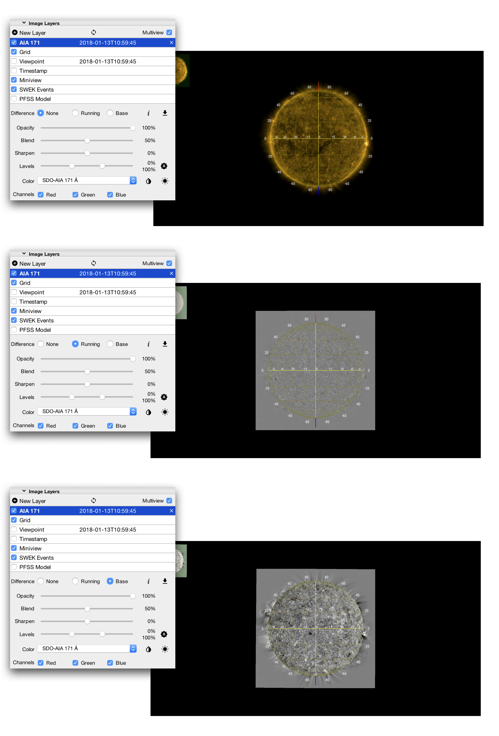
Each layer can be displayed in a difference images mode. Several modes can be selected: “No difference images”, “Running difference” or “Base difference”. No difference images (default) will show the normal image, running difference will subtract the previous image in the sequence from the current image, and base difference will subtract the first image in the sequence from the current image. The figure below shows the result of the two types of difference images compared to the original image.
The opacity, how the image blends with other layers, the perceived sharpness of the image, the low and the high level can also be adjusted. Click between the levels slider thumbs and drag left or right to move together the levels. Double-click to reset the levels. An automatic high level dependent on the content of current image can be calculated by pressing on the “Auto” button. To change the colors used for the image select a different colormap in the dropdown menu. The colors of the image can be inverted by clicking the button next to the colormap dropdown menu. Individual color channels can be turned on and off.
The download button next to the difference image selection combobox allows the download of the data for the selected layer. A JPX file in case of a multiframe layer, or a JP2 file can be found in the Downloads directory of the JHelioviewer home folder.
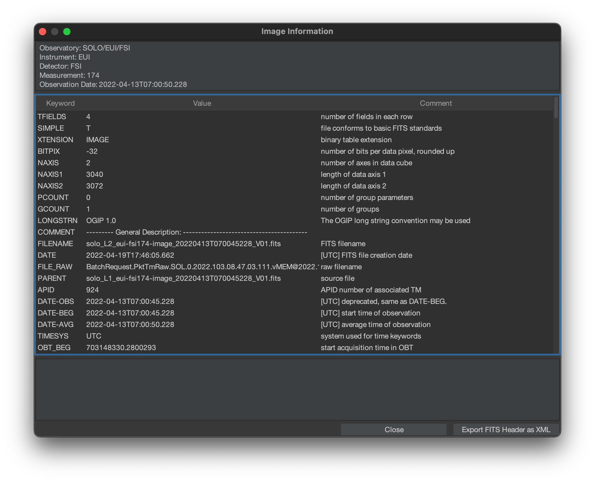
The FITS keywords can be shown by clicking the information icon in the lower right corner of the layer options. Basic information such as the observatory, instrument, detector and observation time, followed by the full list of FITS keywords, are displayed.
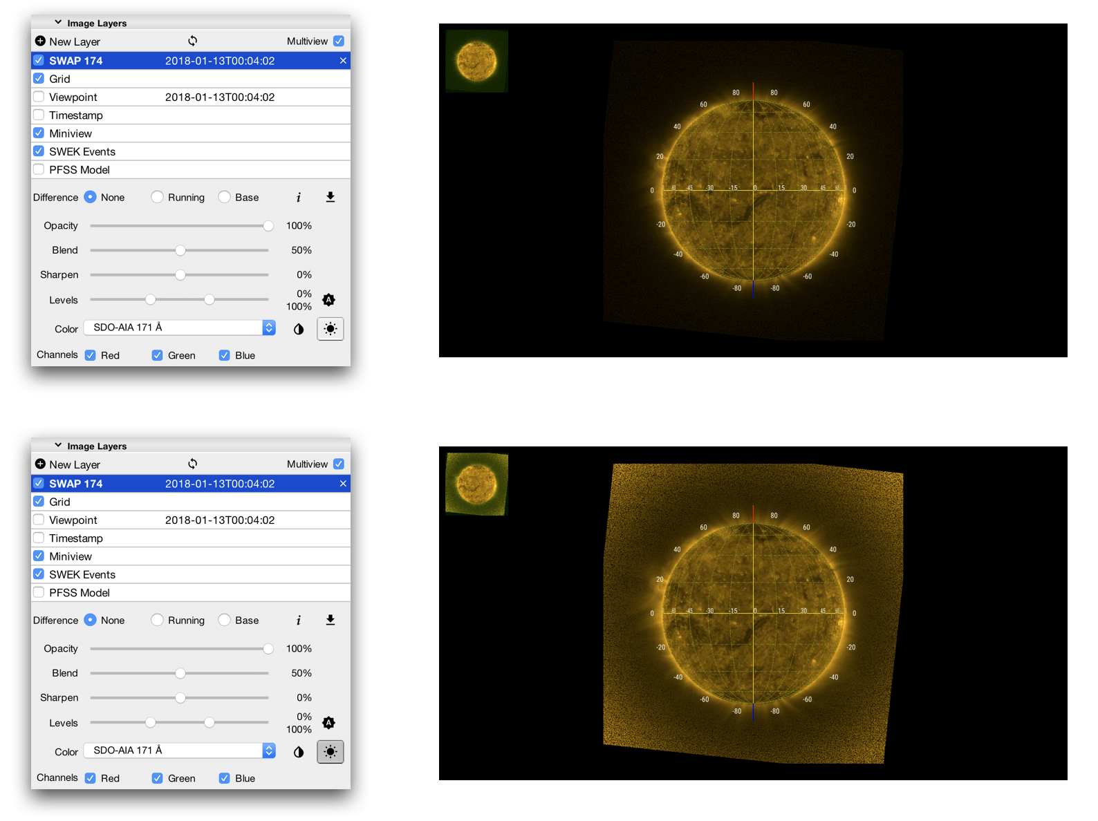
Click the button next to the invert colors button to make the corona better visible as is demonstrated in the enhance corona figure.
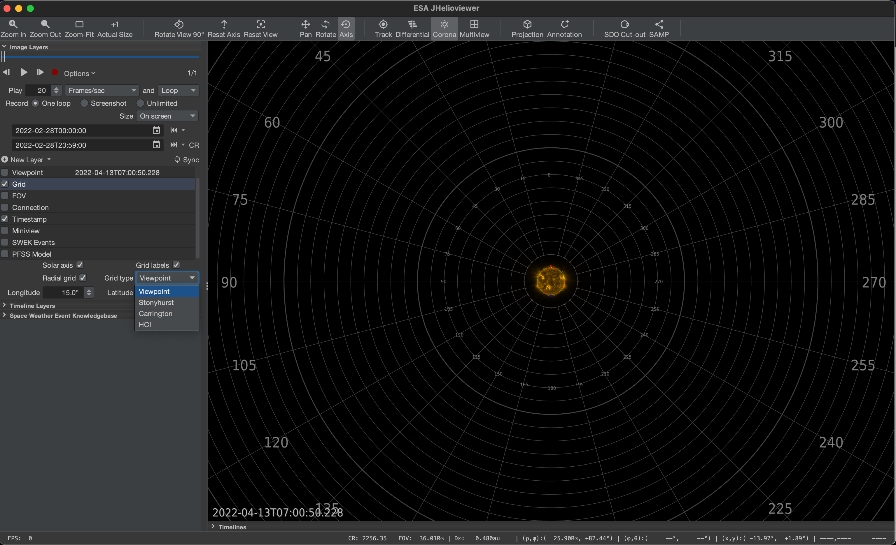
The grid can show heliographic coordinates as seen from the viewpoint, Stonyhurst, Carrington and Heliocentric inertial coordinates. Two yellow great circles indicate the Earth direction and their intersection towards Earth is marked by a point. Clicking the adjacent checkbox can hide the grid. The grid options panel is shown in the figure below. The radial grid can be turned on and off; the same can be done for the solar axis (the blue and red lines at the poles of the Sun) and the grid labels.
The grid ticks size can be changed in both longitude and latitude. The value can be entered directly in the text field, it can be changed by scrolling the mouse over the text field, or by using the arrows. Values ranging from 5˚ and 90˚ are allowed.
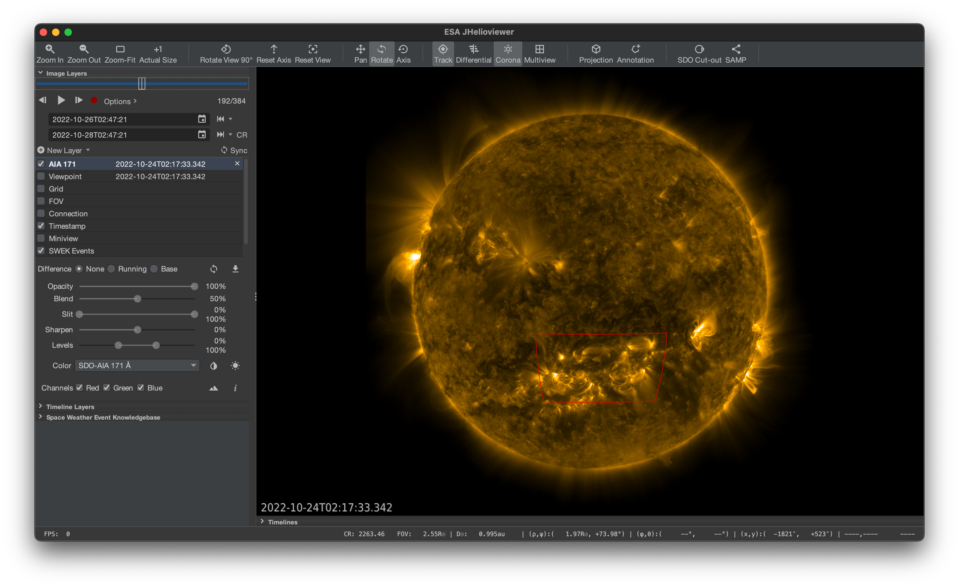
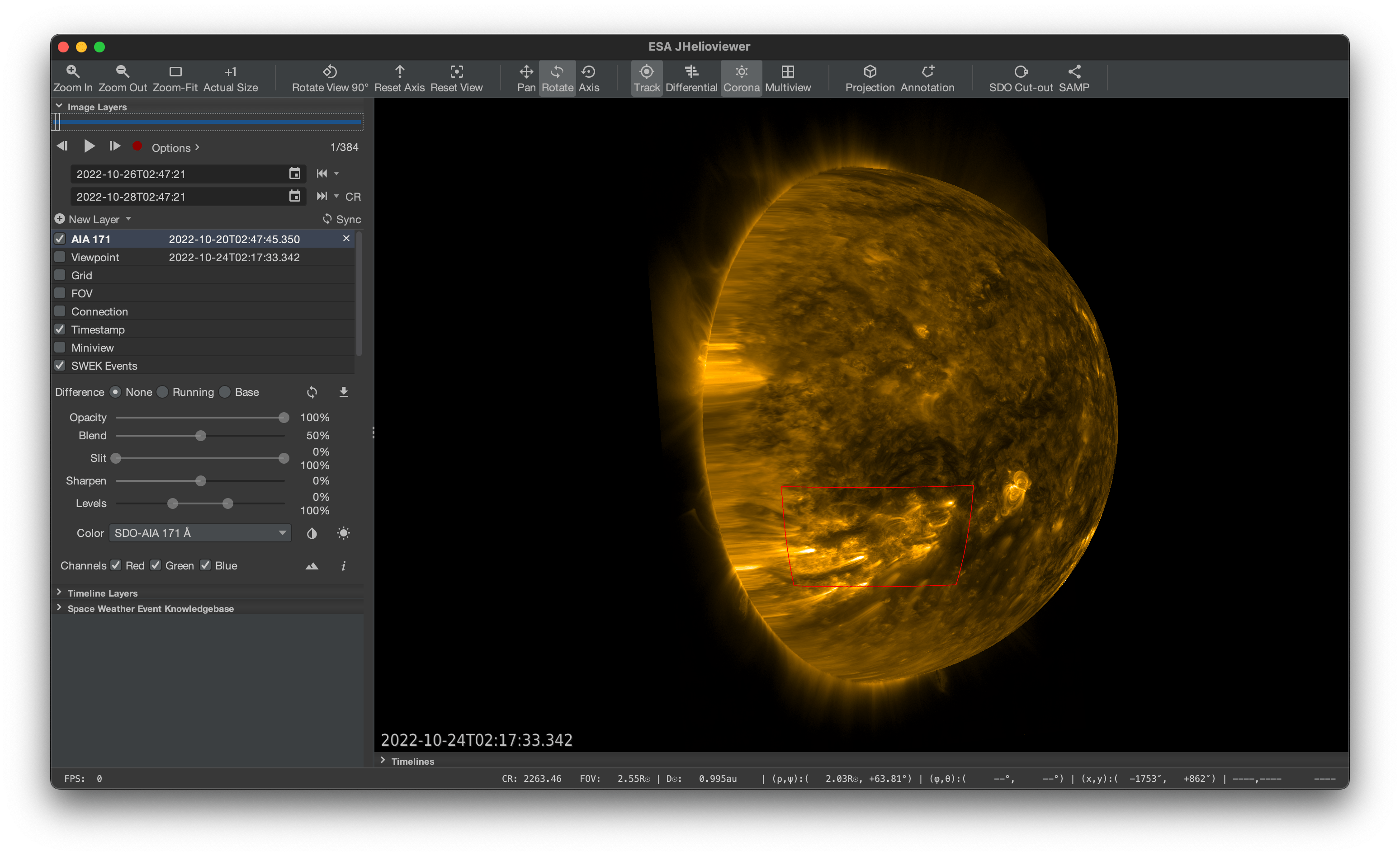
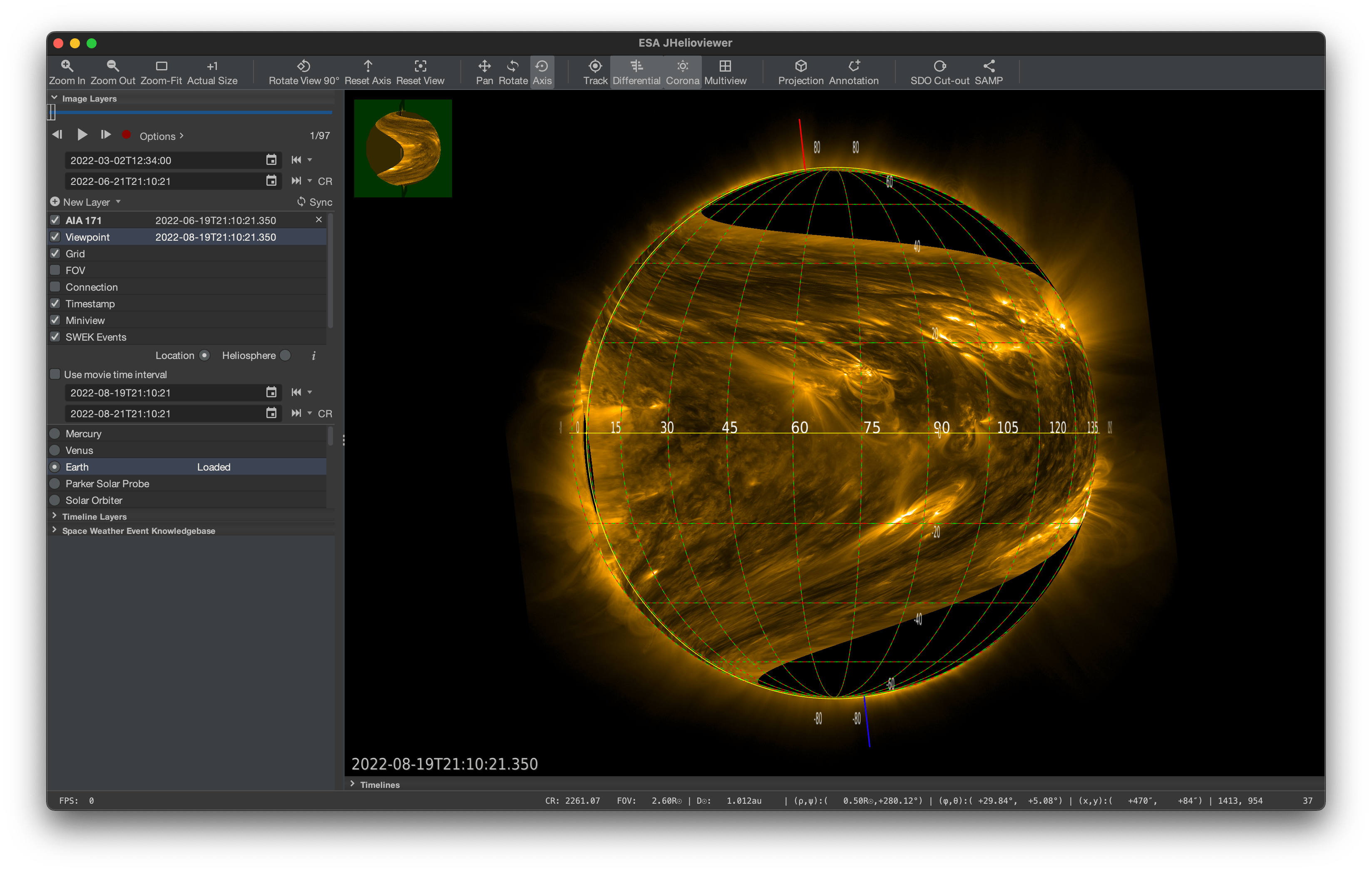
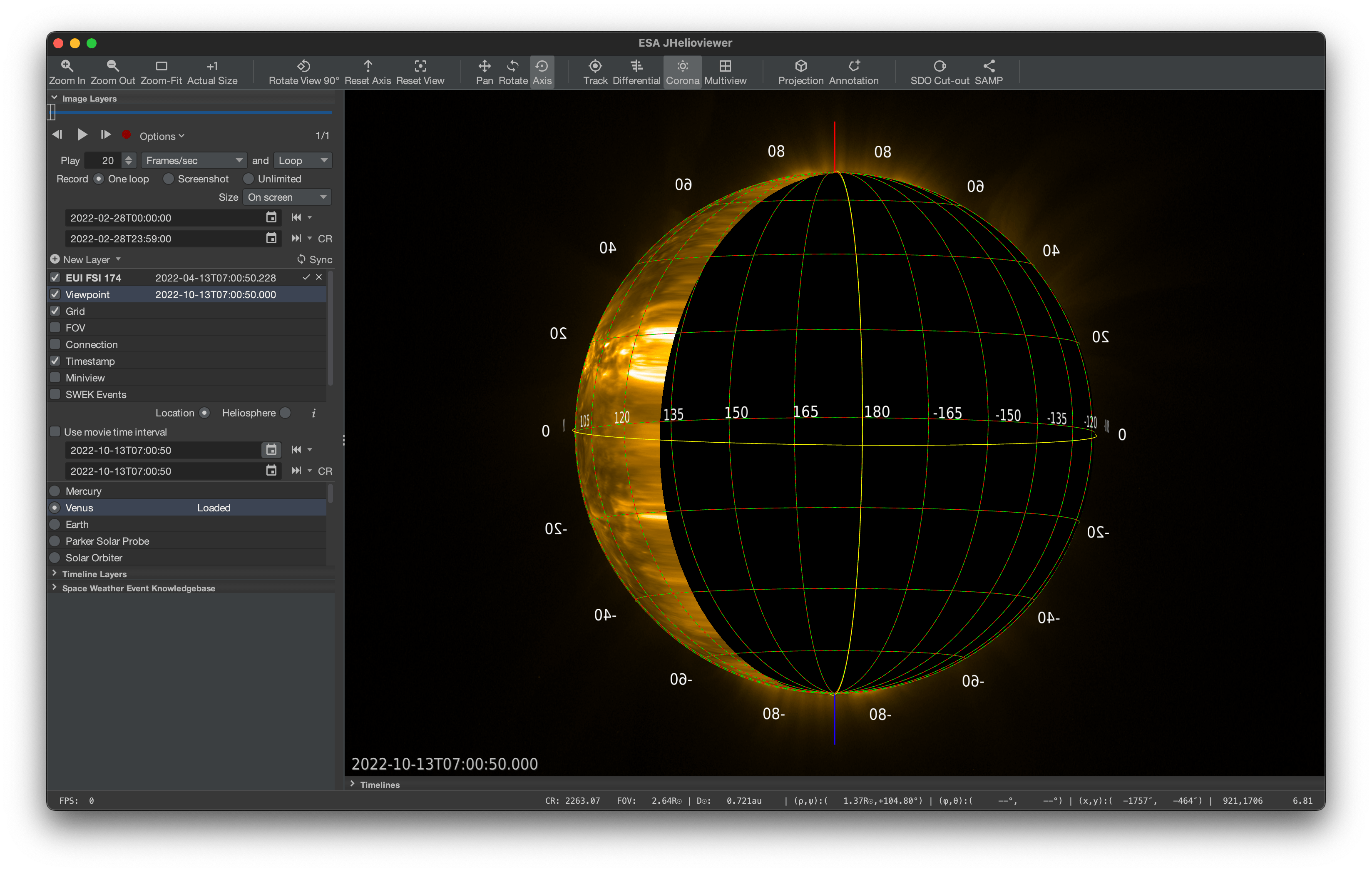
The viewpoint represents the vantage point and is defined by a location in the solar system and a time instance. If the Viewpoint layer is not selected, the scene is viewed as observed. If the layer is selected, the scene is rotated as if it was observed from another location and/or another time, while the images are still correctly placed with respect to the Sun as they were observed.
This is useful to predict the observations of similar instruments from other known vantage points such as planets or spacecraft. It is recommended to use a solar grid linked to the solar rotation such as Carrington or HCI.
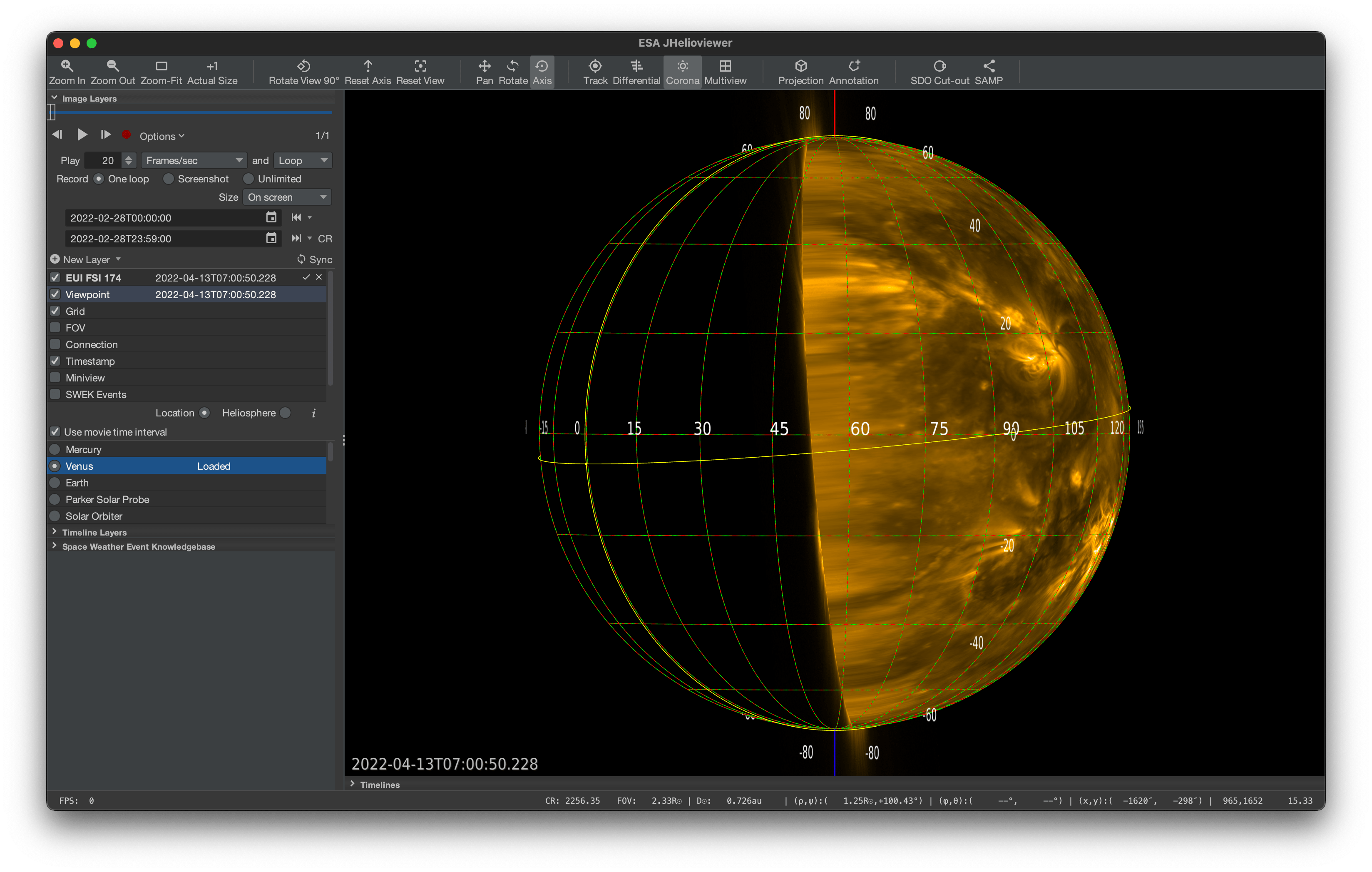
The viewpoint time range can be altered by deselecting Use movie time interval and setting a different time range, for example in the future. The timestamp of the viewpoint is shown in the list of layers.
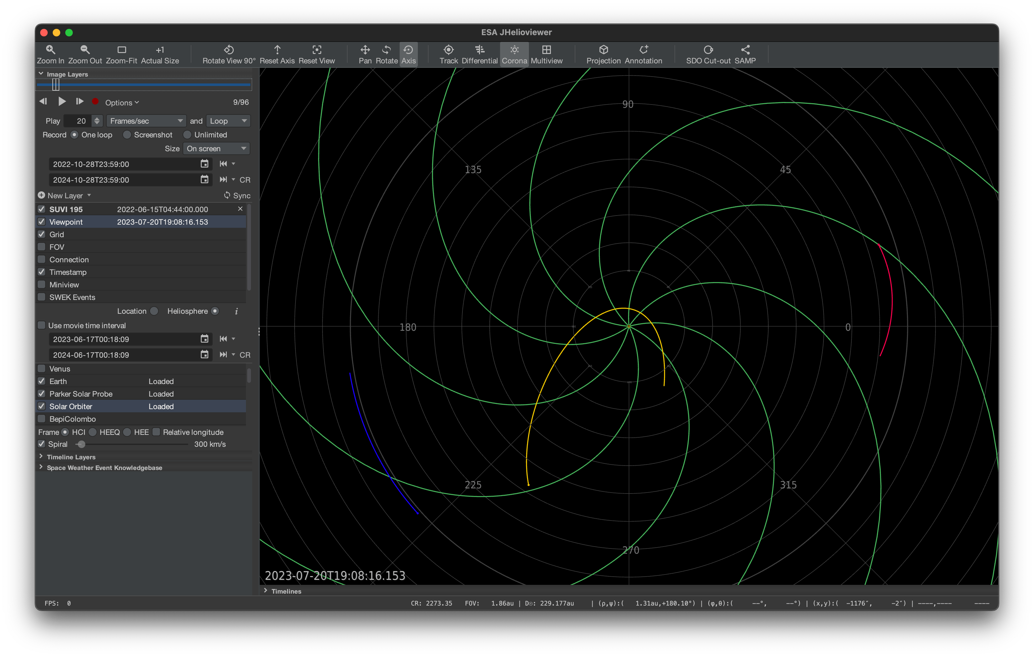
The scene is seen as from above the ecliptic plane and allows the visualisation of orbits. Several reference frames can be selected and the viewing time range can be altered by deselecting Use movie time interval and setting a different time range, for example in the future.
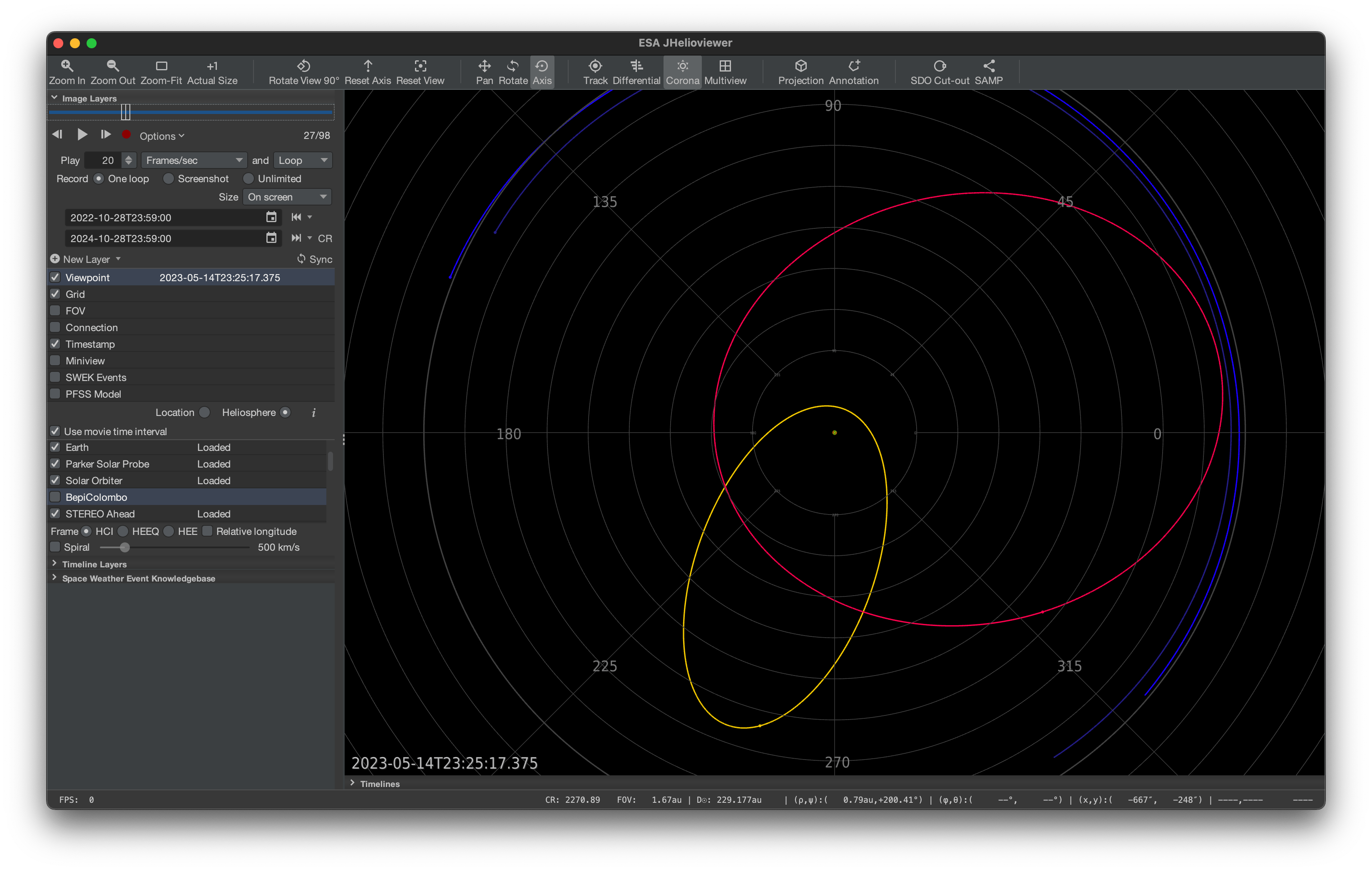
If relative longitude is on, and a particular solar system object is selected from the list, that object is placed at 0 longitude. This allows for an approximate measurement of separation angles in the X-Y plane of the reference frame.
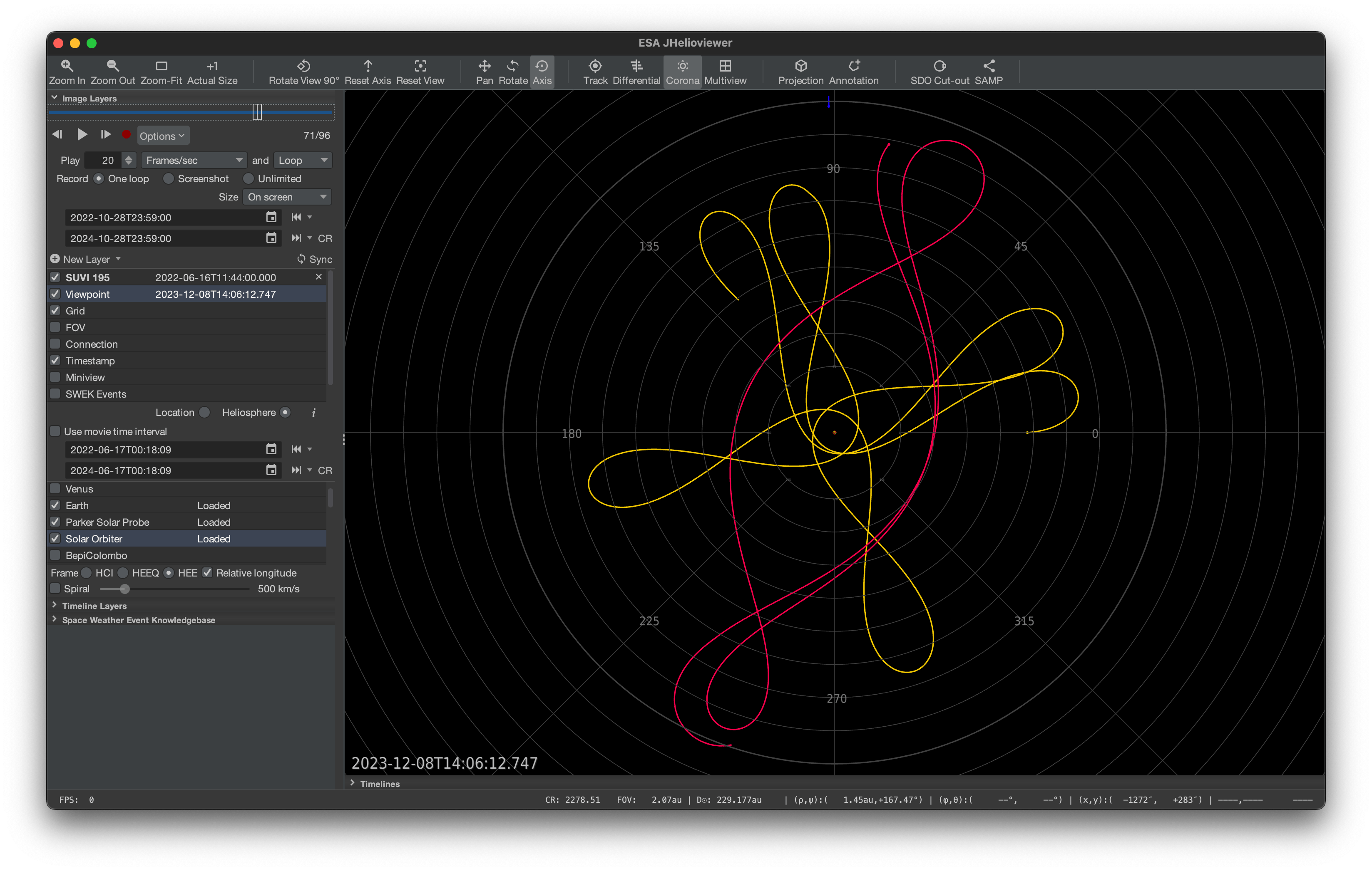
An Archimedean spiral determined by a selectable propagation speed can be drawn. One arm of the spiral will pass through the selected solar system object.
The timestamp layer shows the timestamp of the viewpoint if the multiview mode is off and the timestamps of the individual layers if the multiview mode is on. The text size can be adjusted with a slider, the text can placed at top left and additional information like distance to Sun can be displayed.
The miniview shows a superposition of the loaded image layers irrespective of the current scene which may be substantially zoomed in or out. The size of the miniview can be changed in the option panel with a slider.
The SWEK image layer shows the events that have location information. The events are shown as contours combined with an icon that indicates the type of the event. Events that are on disk are drawn on disk; events like CMEs are drawn as an arch around the Sun. The icons representing the event type can be switched on or off in the options panel. More information can be found in the SWEK section and, in particular, in the section on events on the image canvas.
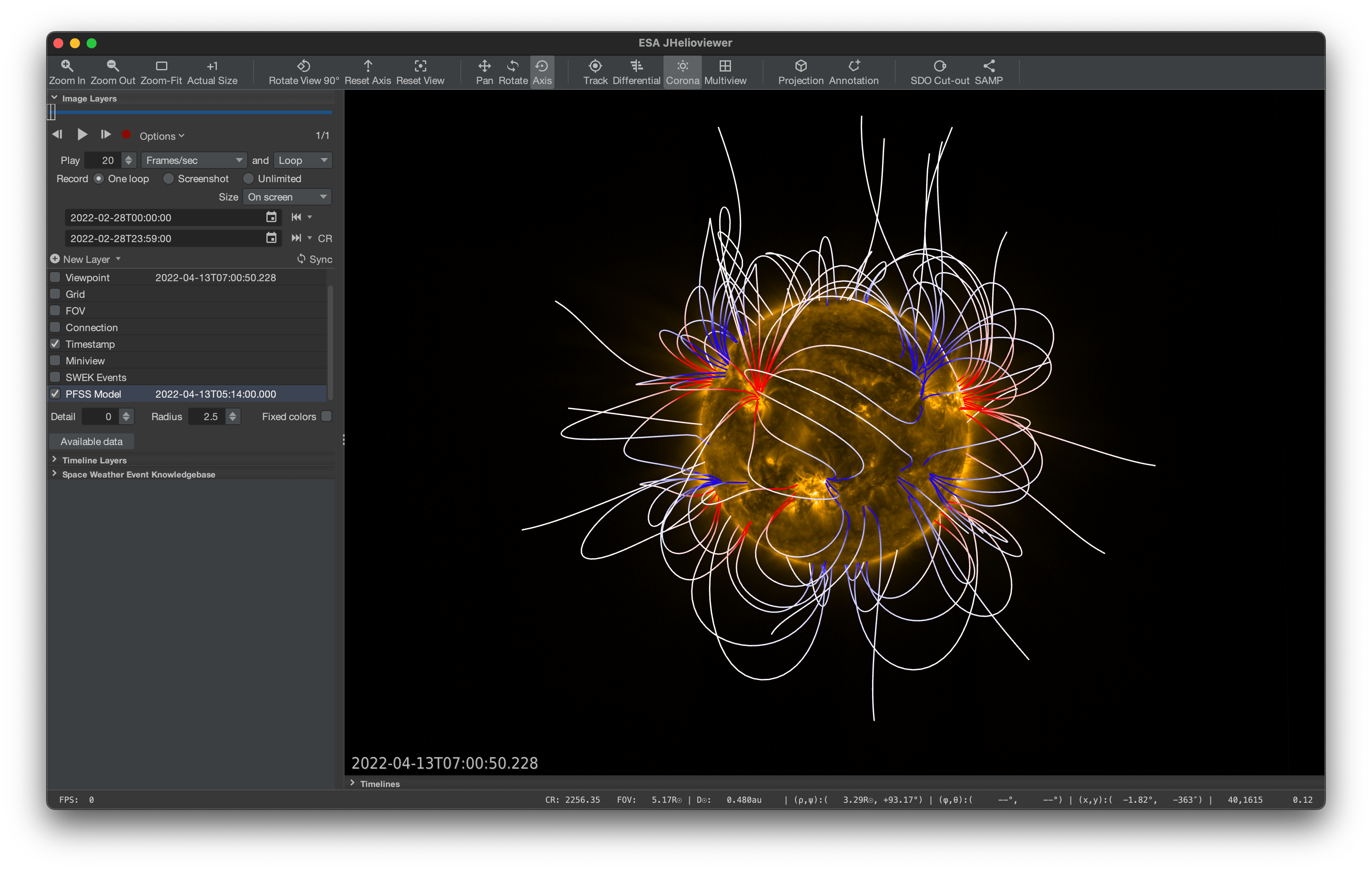
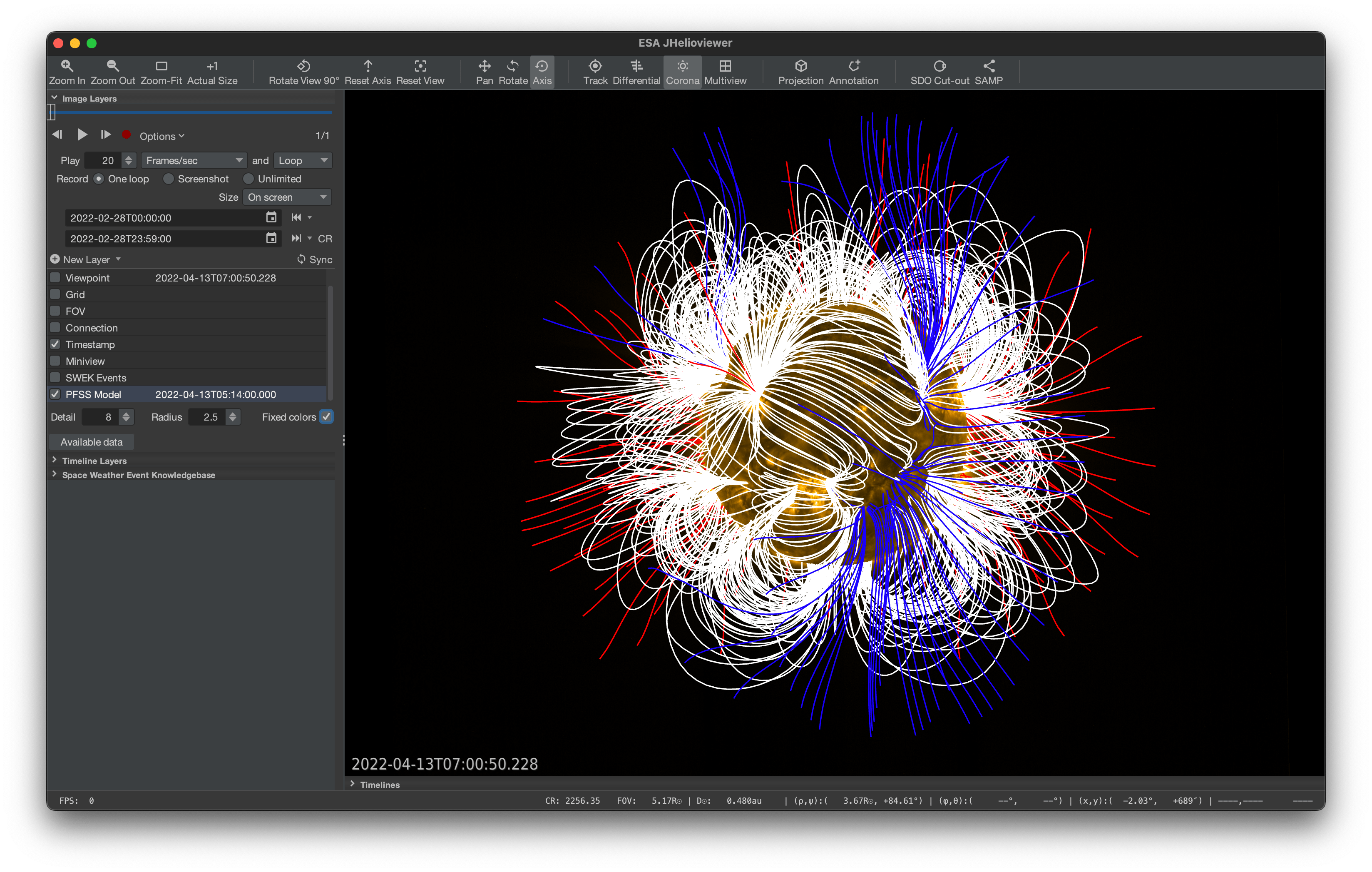
The PFSS model layer visualises a model of the magnetic field derived from magnetograms. The field lines are calculated from GONG magnetograms on the ROB server using a classic model. The timestamp given in the list of layers is the timestamp of the GONG magnetogram used for the calculations. The figures below show different views of the model. The number of field lines shown can be varied by decimation when changing the level of detail between 0 and 8. The radius sets the distance in solar radii that the field lines are visible. By default, the outgoing parts of the field lines are drawn in red, the incoming parts in blue. By enabling the “Fixed colors”, loops will be drawn white, open outgoing field lines red and incoming field lines blue.
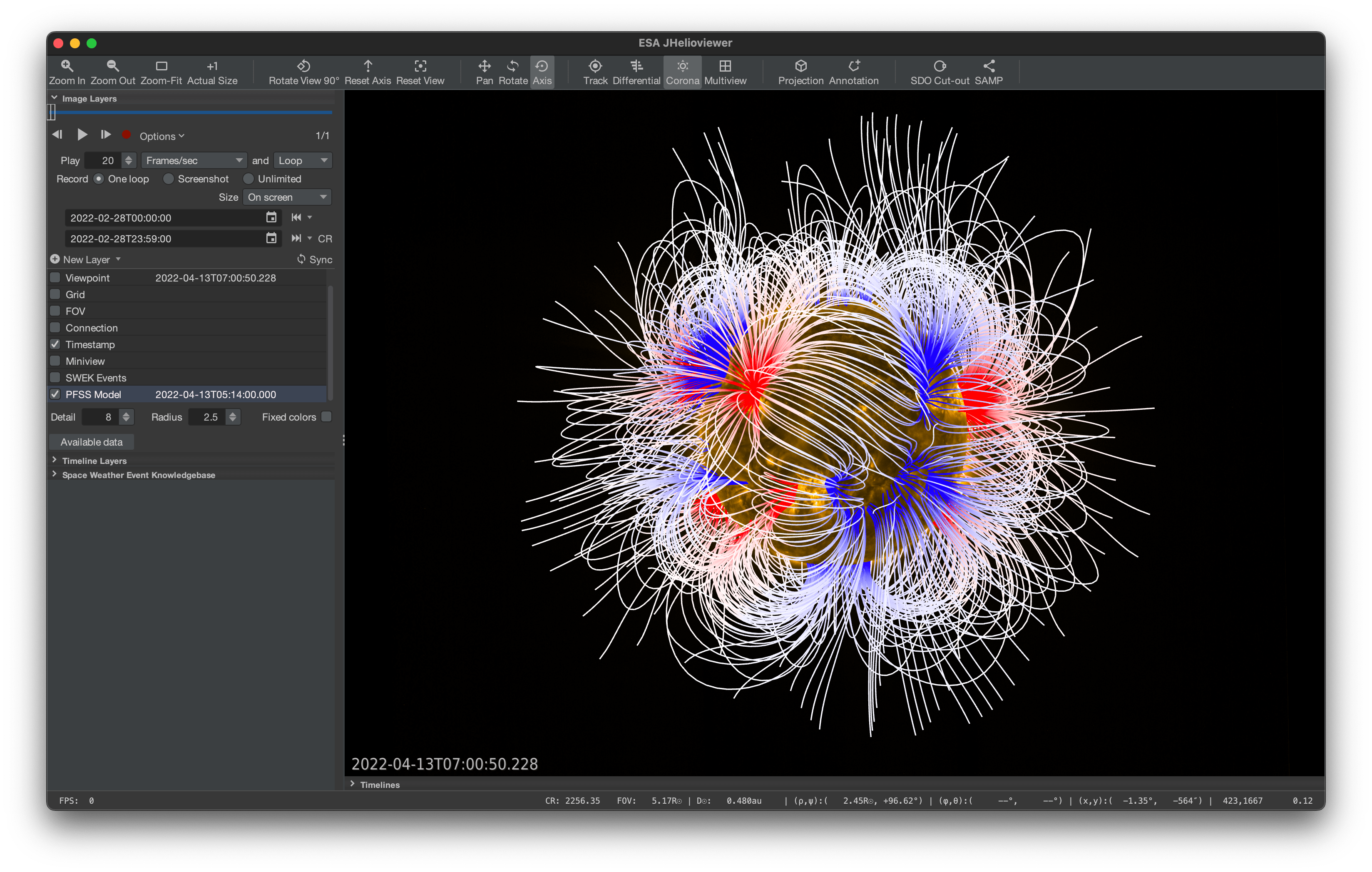
Clicking the “Available data” button brings will open a web browser window with a page showing the available data for the PFSS Model. The darker the green, the more data are available.
JHelioviewer is able to display 1D and 2D timelines. Similar to the images, the timelines have their own panel that lists the timeline layers. The timeline layers can be made visible or invisible. Some timeline layers have options that can be accessed by selecting the corresponding entry in the table listing. The options appear under the listing of the timeline layers.
Timelines can be added and removed. The appearance of the timelines can be changed.
To add a new timeline click the “New Layer” button of the timeline layers panel or the menu item “File>New Timeline…”, select a group and a dataset, and press the “Add” button to add the layer.
A timeline layer can also be added by opening a saved timeline layer via the menu item “File>Open Timeline…”. A file selection dialog will open. Select the wanted timeline layer to be added to the timelines. The missing data will be downloaded automatically. A layer can be removed by clicking the cross. The loading of a layer can be cancelled by clicking the cross while the layer is still loading.
The timeline will be visible in the list of timelines and three days around the chosen date will be downloaded. The timeline will always be given a new y-axis.
A timeline layer can be downloaded by pressing the download layer button in the options panel of the layer.
The availability of timeline datasets can be checked for the ROB server by clicking on the “Available data” button at the bottom left of the dialog box or in the options panel of the timeline. A web browser window will open with a page showing an approximation of the available data on the ROB server. The darker the green, the more data are available.
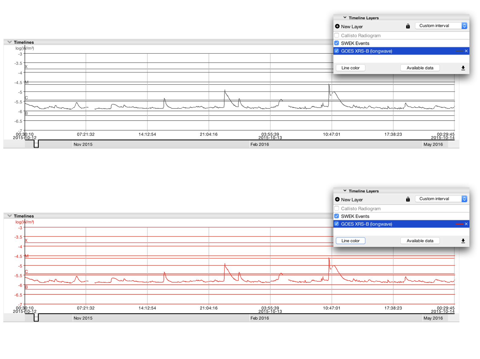
Selecting the timeline and picking a new color with the color picker can change the color for each timeline. This is demonstrated in the figure below.
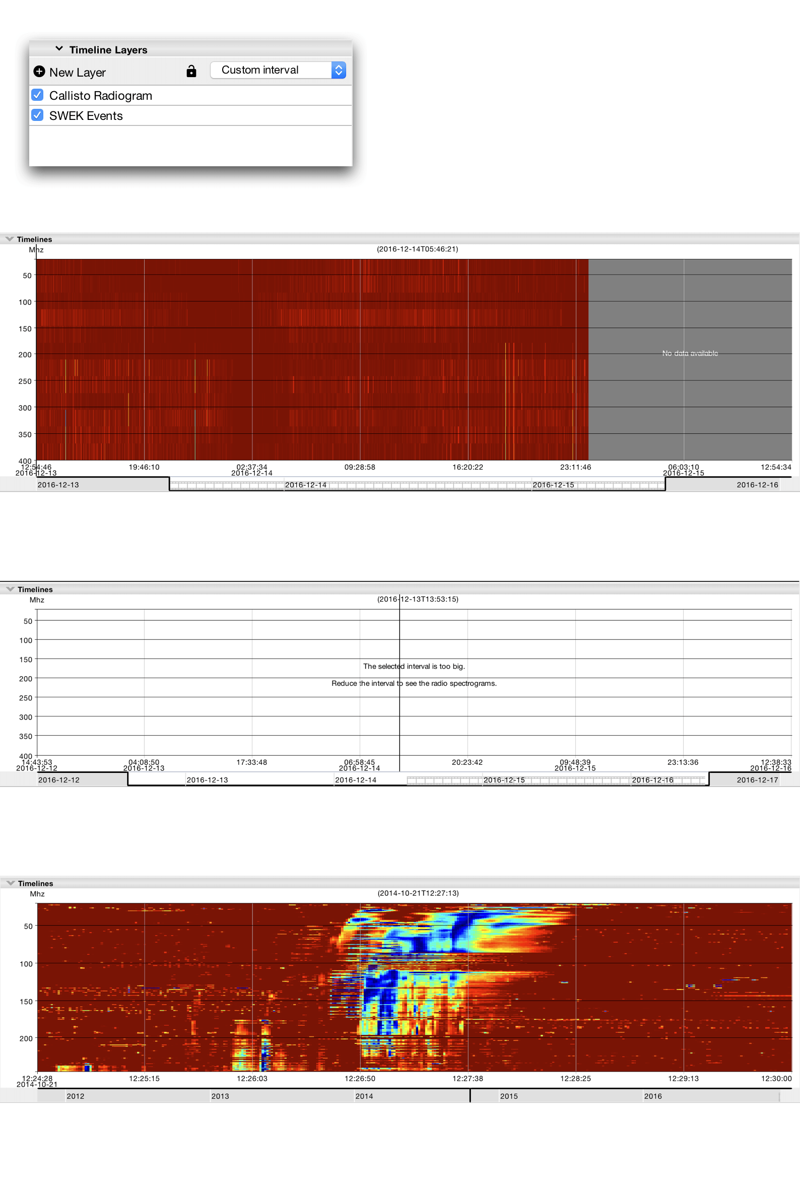
The only two-dimensional data available for the moment are the radio spectra from the global Callisto network of radio receivers. Composite images are created continuously by merging observations from several instruments at different locations, times and frequency bands, therefore the intensity units are arbitrary. The composite images can be shown in the timeline viewer by clicking on the checkbox next to the Callisto Radiogram in the timeline layers panel.
The radio data will appear on the timeline canvas. Images will be grey if the data is loading and if there is no data available. The visible interval should be smaller than three days before the radio data becomes visible. The more zoomed in, the more detail becomes available. This is all demonstrated in the figure below.
The colormap can be changed by selecting the “Callisto Radiogram” in the list of timelines and picking another colormap. The colormaps are listed in the [list of colormaps][colormaps].
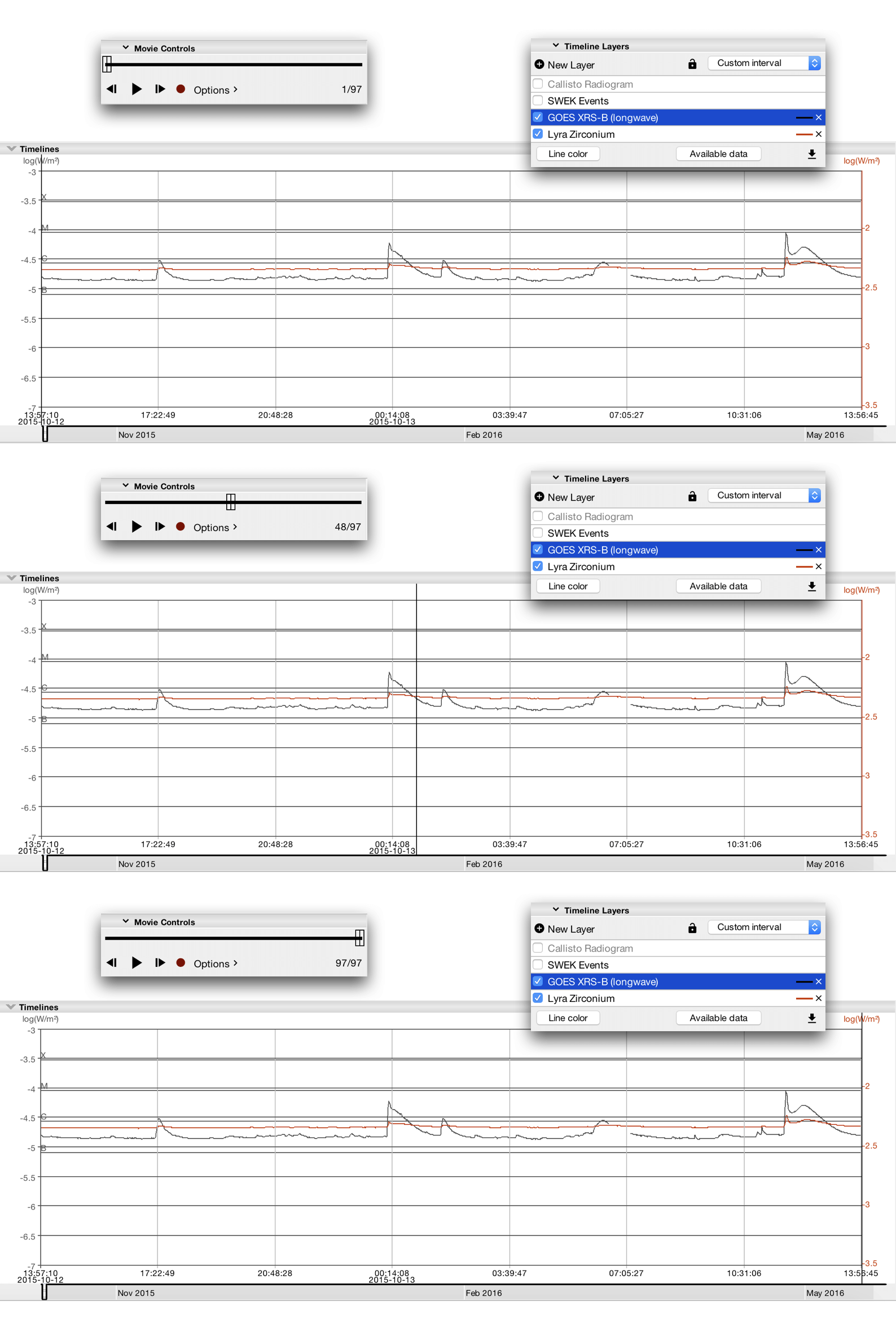
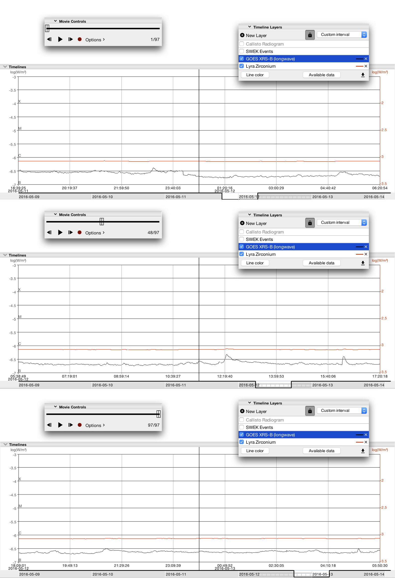
In normal cases, the movie timestamp indicator (vertical black line) will jump towards the correct time as can be seen in the figure with locking mode off. Pressing the lock interval button locks the visible interval of a timeline. Instead of having the visible interval fixed, the interval keeps its width, but the movie indicator will be kept in the middle of the timeline canvas. As a consequence, the data will now slide through the timeline canvas instead of being fixed. This is demonstrated in figure with locking mode on. After the interval lock button was pressed, the visible interval will center around the start of the visible interval. Afterwards, the size of the selected timeline interval can still be adapted as described in the section on timeline canvas manipulation.
The timeline canvas is able to display space weather events. By default space weather events are visible and they can be made invisible by clicking the adjacent checkbox. The events are displayed as colored bars. Events with the same color are related. If the mouse pointer is hovering over an event, that event gets highlighted. More information can be found in the section on events on the timeline canvas.
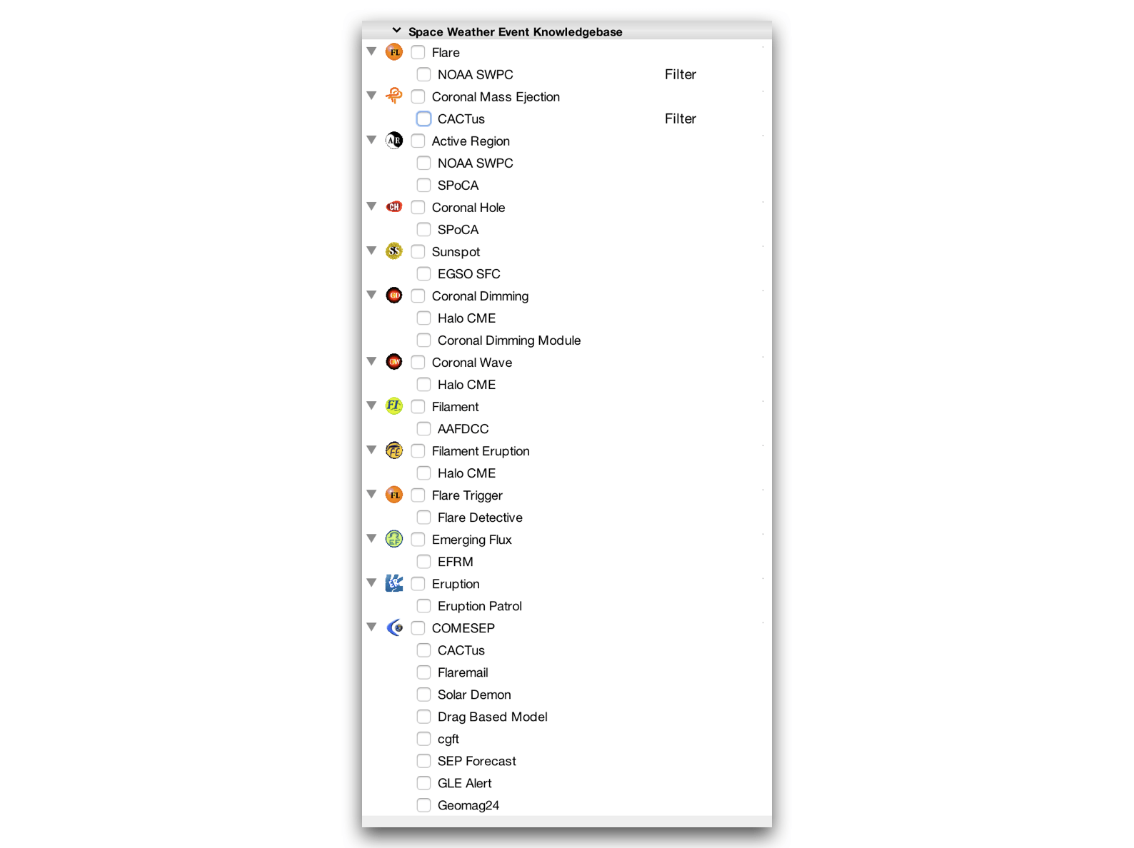
JHelioviewer provides a way to download space weather related events. A selection of important space weather event types was made. The list below enumerates the current default event types.
| Source | Event Type | Provider |
|---|---|---|
| HEK | Active Region | NOAA SWPC |
| SPoCA | ||
| Coronal Mass Ejection | CACTus | |
| Coronal Dimming | Halo CME | |
| Coronal Dimming Module | ||
| Coronal Hole | SPoCA | |
| Coronal Wave | Halo CME | |
| Filament | AAFDCC | |
| Filament Eruption | Halo CME | |
| Flare | NOAA SWPC | |
| Flare Detective | ||
| Sunspot | EGSO SFC | |
| Emerging Flux | EFRM | |
| Plage | ||
| Eruption | Eruption Patrol | |
| COMESEP | COMESEP | CACTus |
| Flaremail | ||
| Solar Demon | ||
| Drag Based Model | ||
| CGFT | ||
| SEP Forecast | ||
| GLE Alert | ||
| Geomag24 |
For the moment only two sources for events are used: the Heliophysics Events Knowledgebase (HEK) and the COMESEP alert system.
By checking or unchecking the checkbox next to the event provider, or to the event type, the event types are enabled or disabled, as shown in the figure below. Once an event or event type is enabled, the download for the selected interval will start. Events that were downloaded are kept in a cache. Enabling and disabling events only initiate a new download of the events for the last two weeks.
Some events can be filtered:
- click the “Filter” button next to the event type to filter,
- set the values for the filter,
- switch the filter button on,
- the event type will be filtered.
Just switch off the filter button to remove the filter.
Space weather events are displayed by means of contours in the color of the event, and an icon of the event type on the image canvas (see the figure of events on both canvases). The event will only be visible if it contains location information. Not all the events have location information. By hovering with the mouse pointer over the events in the image canvas, the event gets highlighted and some brief information about it will be shown next to the mouse pointer. If the event is visible in the timeline canvas, it will be highlighted too. An event information dialog will appear after clicking on the icon.
The events can be made visible or invisible by clicking the checkbox in the image layers list as described in the section on image layers panel.
Events are displayed as colored bars in the timeline canvas (see the figure of events on both canvases). Related events have the same color and if possible, aligned at the same height level. Events are grouped by event type. By hovering with the mouse pointer over the events, the events get highlighted. The event information dialog will be displayed after clicking on the event.
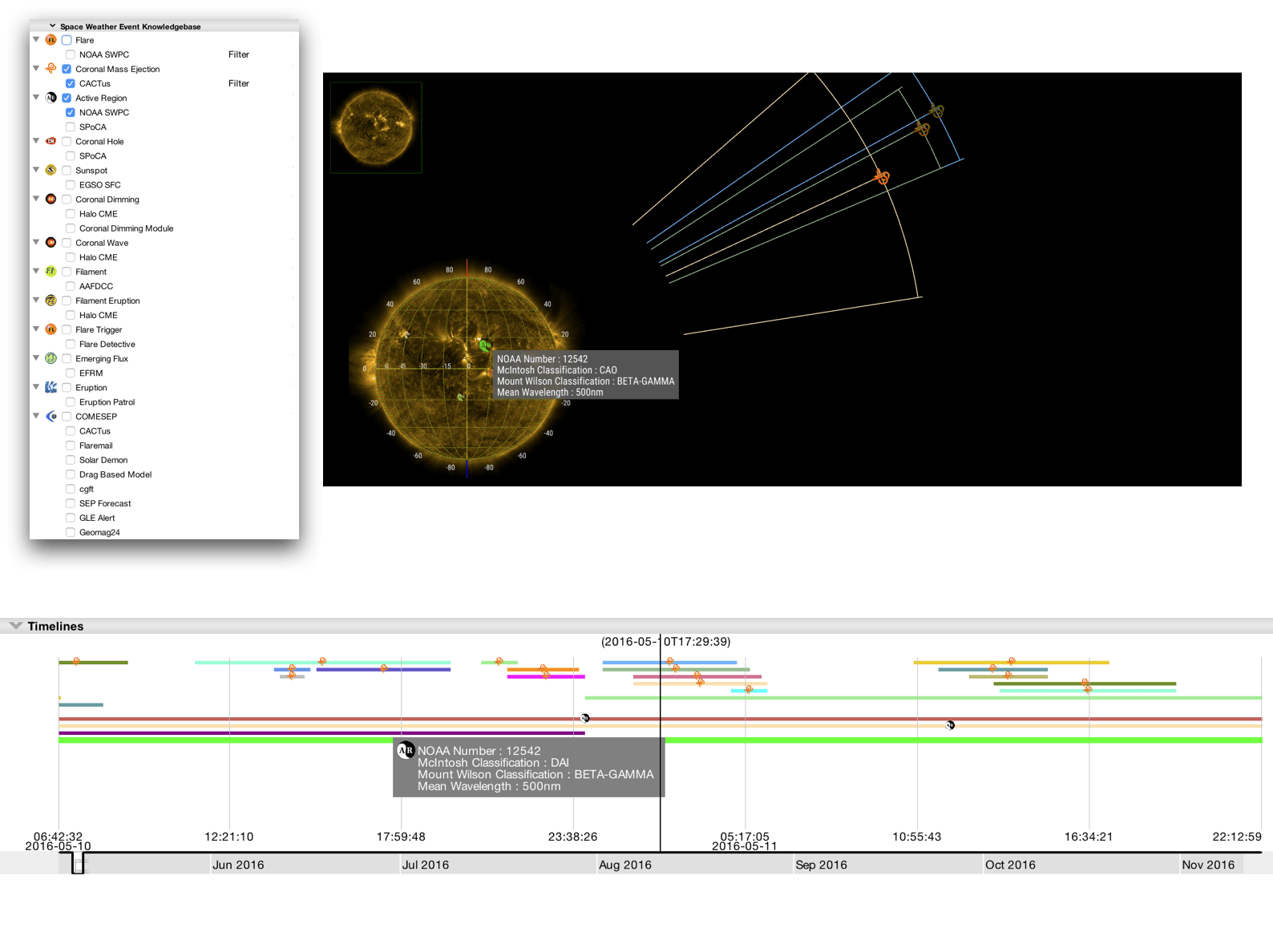
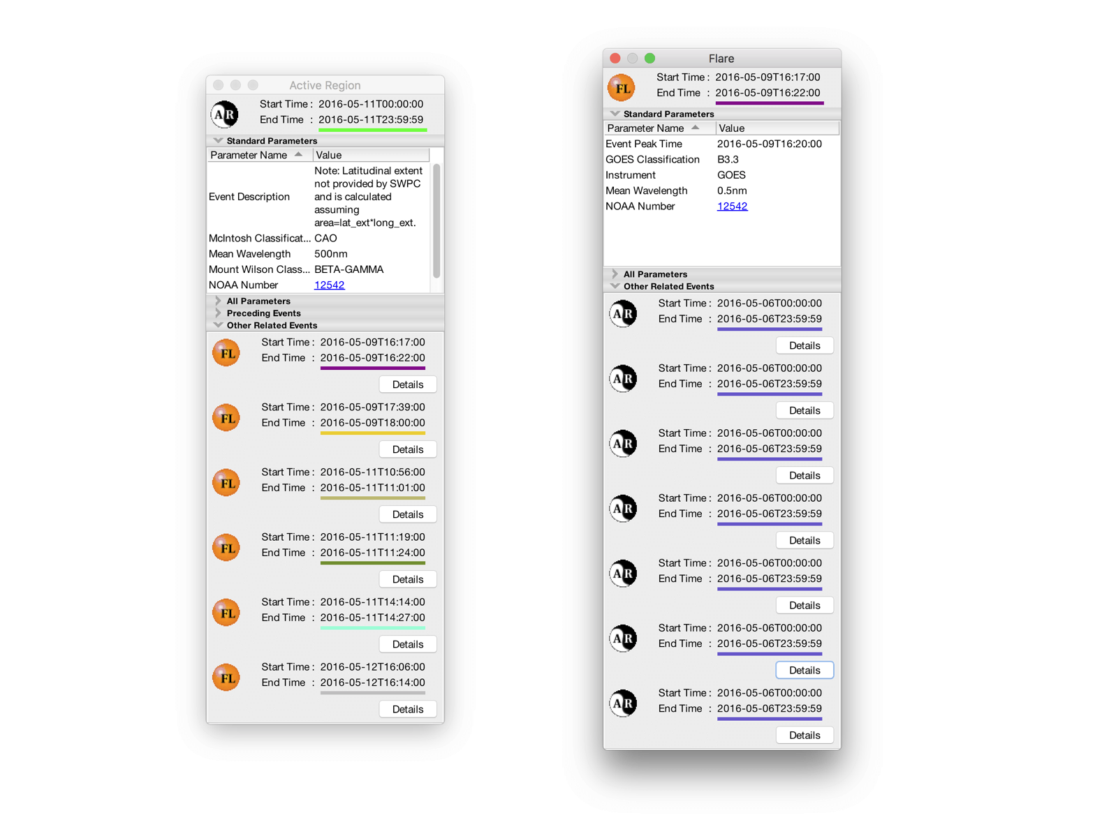
Each event has details that become visible after clicking on the event in the image canvas or the timeline canvas. A dialog box will appear with the detailed information of the event. The title of the dialog box together with the icon defines the event type. The start and end time of the event are given, together with a patch in the color used for the event. To locate the event in the canvases, hovering with the mouse pointer over the icon and the colored patch will highlight the event.
An event has a standard and an all parameters panel. The standard parameters are parameters that are the most important for the event. The all parameters panel contains a list of all the parameters returned by the event provider that contained a valid value. An http link as the value of a parameter is clickable and will open in the browser. Some parameters might be clickable and allow to search for papers mentioning this parameter and event.
The event information dialog can also contain relationship information. Three different relationships exist:
Some event providers send their events each day and also link them together. This is the case for active regions or coronal holes detected by SPoCA. The preceding and following events will get the same color. This is shown on the right part of the figure of detail dialog box for SPoCA active region events.
Some events are related by rules. The active region number provides the relationship between active regions and flares. If both the event types flare and active region are enabled and a flare has the same active region number as an active region, this relationship will be visible in the “Related by rule”-panel. This is shown on the left part of the figure of detail dialog box.
The related events panels contain a list of small panels containing for each of the related event the icon of the event type and the color. If the events are in view in the image or the timeline canvas, hovering with the mouse pointer over this panel will highlight the related event.
The image and timeline canvases can be exported in three ways: a one-loop movie, a screenshot, or an open ended recording of all the manipulations. All movies are saved in the directory JHelioviewer-SWHV/Exports/ in the home directory. The export format can be set in the preferences. The movies can be either a streamable MP4 container file or series of PNGs. The MP4 files can be in H.264/AVC format for better compatibility or in H.265/HEVC for smaller files. Screenshots are saved in the PNG format. Several frame sizes are offered: from the image canvas original size (on screen) and up to 4096 by 4096. The exported movie file has the selected frames per second setting.
The record button is in the movie control panel. The default recording mode is a one-loop movie of the selected visible image layers together with the timeline canvas if visible. The created movie file will contain the first until the last frame of the current movie. The screenshot mode will make a screenshot of the current image and timeline canvases. In unlimited mode, all the manipulations are recorded from the moment the record button is clicked. Clicking the same record button, now indicating “busy”, stops the recording. Removing all image layers also stops the recording.
The state file captures all the program’s presentation including the loaded remote data, its orientation, and the options of the layers. This can be used to quickly reproduce a particular solar event or to share a particular combined presentation of data. The state file is a JSON file which can be saved by selecting “File>Save State” and loaded by “File>Load State…”.
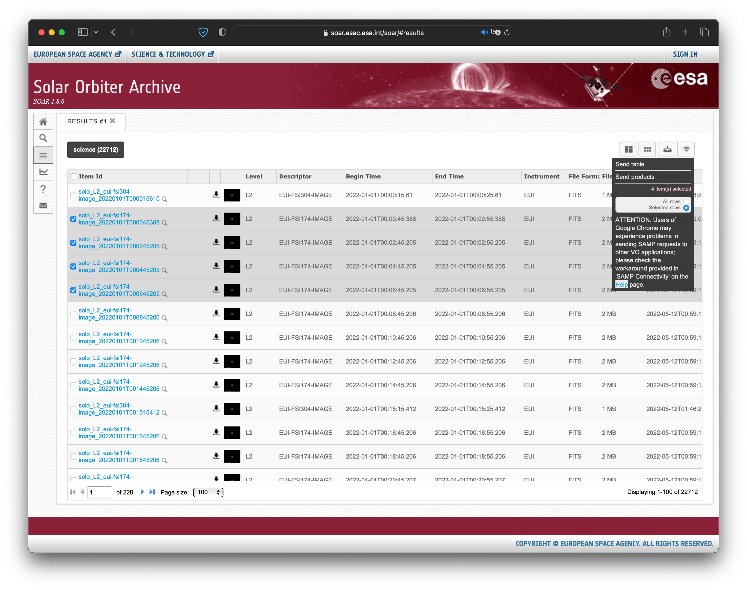
SAMP is an inter-application messaging protocol standardised by IVOA that enables astronomy software tools to interoperate and communicate. The GitHub samp4jhv project contains a collection of examples on how data can be shared between JHelioviewer and Python or IDL environments.
This protocol can also be used on the web and the figure below shows the online SOAR archive which can send FITS and CDF files to JHelioviewer. Selecting “Send table” will instruct JHelioviewer to load the selected FITS files as a movie. Selecting “Send products” will make JHelioviewer to load the selected files as different layers.
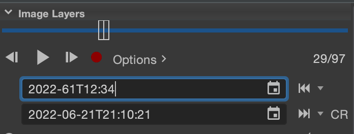
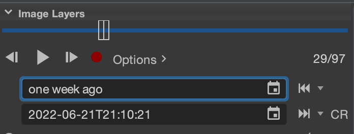
All time input and display in JHelioviewer is UTC in ISO8601 format. Day of year format is supported, as well as natural English language phrases such as “one year ago” or “two weeks ago”. If the input is not recognized or if the start time is later than the end time, the time field reverts to previously displayed value. The entire time range can be shifted backward or forward with a selectable duration (day/week/Carrington rotation). The period of an entire Carrington rotation can be filled in the time fields by clicking the “CR” button.
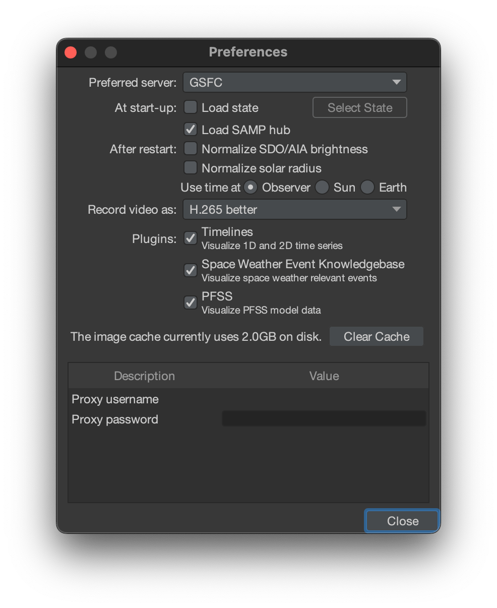
The preferences dialog can be found under the program menu (JHelioviewer) on macOS, for Windows and Linux it is located in the menu “Options”. A new dialog opens. The following persistent options can be set:
Several parts of the interface can be turned on and off under the Plugins heading: Timelines/SWEK/PFSS. The persistent image cache can also be cleared, as well as a proxy username and password can be set if required.
| Operation | Key combination |
|---|---|
| Add new layer | Cmd/Ctrl-N |
| Open file | Cmd/Ctrl-O |
| Toggle full screen | Cmd/Ctrl-Enter |
| Exit full screen | Esc |
| Actual size | Cmd/Ctrl–0 |
| Zoom to fit | Cmd/Ctrl–9 |
| Zoom in | Cmd/Ctrl-= |
| Zoom out | Cmd/Ctrl– |
| Play movie | Cmd/Ctrl-P |
| Step to previous frame | Cmd/Ctrl-Alt-Left Arrow |
| Step to next frame | Cmd/Ctrl-Alt-Right Arrow |
| Remove current annotation | Shift- Delete/Backspace |
| Cycle through annotations | Shift- n(ext)/p(revious) |
| Operation | Action |
|---|---|
| Double-click | Reset Camera |
| Scroll Up | Zoom Out |
| Scroll Down | Zoom In |
| Click and Drag | Pan in Panning Mode |
| Rotate in Rotation Mode | |
| Shift-click and Drag | Enter annotation mode and draw; release mouse button then the shift key to exit mode |
| Right-click | Copy to clipboard the position data at the mouse pointer |
| Operation | Action |
|---|---|
| Double-click on Graph | Rescale Graphs Between Minimum and Maximum values |
| Double-click on Axis | Rescale Graphs Between Default Minimum and Maximum value |
| Scroll Up on Graph | Zoom Out in Time |
| Scroll Down on Graph | Zoom In in Time |
| Scroll Up on Value-Axis | Zoom Out in Value |
| Scroll Down on Value-Axis | Zoom In in Value |
| Scroll Up on Time-Axis | Zoom Out in Value And Time |
| Scroll Down on Time-Axis | Zoom In in Value And Time |
| Shift-Scroll Up on Graph area | Move Forward in Time with Same Visible Interval |
| Shift-Scroll Down on Graph area | Move Backward in Time with Same Visible Interval |
| Ctrl-Scroll Up | Zoom Out in Time and Value |
| Alt-scroll Up | |
| Ctrl-Scroll Down | Zoom In in Time and Value |
| Alt-Scroll Down | |
| Click | Move Movie Time Indicator |
| Click and Drag on Graph | Move Graph in Time and Value |
| Click and Drag on Value-Axis | Move Graph in Value |
Although a lot of effort was put into reducing the memory usage of JHelioviewer, it occasionally may run out of the default amount reserved by Java. The amount of memory reserved by Java can be tweaked from the command line.
To start JHelioviewer from the command line in Windows:
cmd
cd "C:\Program Files\JHelioviewer\classes"
..\jre\bin\java.exe -Xmx4g --add-exports java.desktop/sun.awt=ALL-UNNAMED --add-exports java.desktop/sun.swing=ALL-UNNAMED -cp JHelioviewer.jar;natives-windows.jar org.helioviewer.jhv.JHelioviewer
or where is JHelioviewer installed.
This allocates maximum 4GB for Java and reduces the risk of running into out-of-memory errors.
To find the amount of memory allocated by Java type:
"C:\Program Files\JHelioviewer\jre\bin\java.exe" -XX:+PrintFlagsFinal -version | findstr /R /C:"HeapSize"
The interesting value is MaxHeapSize.